Note
Go to the end to download the full example code or to run this example in your browser via JupyterLite or Binder.
Class Likelihood Ratios to measure classification performance#
This example demonstrates the class_likelihood_ratios
function, which computes the positive and negative likelihood ratios (LR+,
LR-) to assess the predictive power of a binary classifier. As we will see,
these metrics are independent of the proportion between classes in the test set,
which makes them very useful when the available data for a study has a different
class proportion than the target application.
A typical use is a case-control study in medicine, which has nearly balanced classes while the general population has large class imbalance. In such application, the pre-test probability of an individual having the target condition can be chosen to be the prevalence, i.e. the proportion of a particular population found to be affected by a medical condition. The post-test probabilities represent then the probability that the condition is truly present given a positive test result.
In this example we first discuss the link between pre-test and post-test odds given by the Class likelihood ratios. Then we evaluate their behavior in some controlled scenarios. In the last section we plot them as a function of the prevalence of the positive class.
# Authors: The scikit-learn developers
# SPDX-License-Identifier: BSD-3-Clause
Pre-test vs. post-test analysis#
Suppose we have a population of subjects with physiological measurements X
that can hopefully serve as indirect bio-markers of the disease and actual
disease indicators y (ground truth). Most of the people in the population do
not carry the disease but a minority (in this case around 10%) does:
from sklearn.datasets import make_classification

X, y = make_classification(n_samples=10_000, weights=[0.9, 0.1], random_state=0)
print(f"Percentage of people carrying the disease: {100 * y.mean():.2f}%")
Percentage of people carrying the disease: 10.37%
A machine learning model is built to diagnose if a person with some given physiological measurements is likely to carry the disease of interest. To evaluate the model, we need to assess its performance on a held-out test set:
from sklearn.model_selection import train_test_split

X_train, X_test, y_train, y_test = train_test_split(X, y, random_state=0)
Then we can fit our diagnosis model and compute the positive likelihood ratio to evaluate the usefulness of this classifier as a disease diagnosis tool:
from sklearn.linear_model import LogisticRegression
from sklearn.metrics import class_likelihood_ratios

estimator = LogisticRegression().fit(X_train, y_train)
y_pred = estimator.predict(X_test)
pos_LR, neg_LR = class_likelihood_ratios(y_test, y_pred, replace_undefined_by=1.0)
print(f"LR+: {pos_LR:.3f}")
LR+: 12.617
Since the positive class likelihood ratio is much larger than 1.0, it means that the machine learning-based diagnosis tool is useful: the post-test odds that the condition is truly present given a positive test result are more than 12 times larger than the pre-test odds.
Cross-validation of likelihood ratios#
We assess the variability of the measurements for the class likelihood ratios in some particular cases.
import pandas as pd


def scoring(estimator, X, y):
    y_pred = estimator.predict(X)
    pos_lr, neg_lr = class_likelihood_ratios(y, y_pred, replace_undefined_by=1.0)
    return {"positive_likelihood_ratio": pos_lr, "negative_likelihood_ratio": neg_lr}


def extract_score(cv_results):
    lr = pd.DataFrame(
        {
            "positive": cv_results["test_positive_likelihood_ratio"],
            "negative": cv_results["test_negative_likelihood_ratio"],
        }
    )
    return lr.aggregate(["mean", "std"])
We first validate the LogisticRegression model
with default hyperparameters as used in the previous section.
from sklearn.model_selection import cross_validate

estimator = LogisticRegression()
extract_score(cross_validate(estimator, X, y, scoring=scoring, cv=10))
We confirm that the model is useful: the post-test odds are between 12 and 20 times larger than the pre-test odds.
On the contrary, let’s consider a dummy model that will output random predictions with similar odds as the average disease prevalence in the training set:
from sklearn.dummy import DummyClassifier

estimator = DummyClassifier(strategy="stratified", random_state=1234)
extract_score(cross_validate(estimator, X, y, scoring=scoring, cv=10))
Here both class likelihood ratios are compatible with 1.0 which makes this classifier useless as a diagnostic tool to improve disease detection.
Another option for the dummy model is to always predict the most frequent class, which in this case is “no-disease”.
estimator = DummyClassifier(strategy="most_frequent")
extract_score(cross_validate(estimator, X, y, scoring=scoring, cv=10))
/home/circleci/project/sklearn/utils/_param_validation.py:218: UndefinedMetricWarning: No samples were predicted for the positive class and `positive_likelihood_ratio` is set to `np.nan`. Use the `replace_undefined_by` param to
  return func(*args, **kwargs)
/home/circleci/project/sklearn/utils/_param_validation.py:218: UndefinedMetricWarning: No samples were predicted for the positive class and `positive_likelihood_ratio` is set to `np.nan`. Use the `replace_undefined_by` param to
  return func(*args, **kwargs)
/home/circleci/project/sklearn/utils/_param_validation.py:218: UndefinedMetricWarning: No samples were predicted for the positive class and `positive_likelihood_ratio` is set to `np.nan`. Use the `replace_undefined_by` param to
  return func(*args, **kwargs)
/home/circleci/project/sklearn/utils/_param_validation.py:218: UndefinedMetricWarning: No samples were predicted for the positive class and `positive_likelihood_ratio` is set to `np.nan`. Use the `replace_undefined_by` param to
  return func(*args, **kwargs)
/home/circleci/project/sklearn/utils/_param_validation.py:218: UndefinedMetricWarning: No samples were predicted for the positive class and `positive_likelihood_ratio` is set to `np.nan`. Use the `replace_undefined_by` param to
  return func(*args, **kwargs)
/home/circleci/project/sklearn/utils/_param_validation.py:218: UndefinedMetricWarning: No samples were predicted for the positive class and `positive_likelihood_ratio` is set to `np.nan`. Use the `replace_undefined_by` param to
  return func(*args, **kwargs)
/home/circleci/project/sklearn/utils/_param_validation.py:218: UndefinedMetricWarning: No samples were predicted for the positive class and `positive_likelihood_ratio` is set to `np.nan`. Use the `replace_undefined_by` param to
  return func(*args, **kwargs)
/home/circleci/project/sklearn/utils/_param_validation.py:218: UndefinedMetricWarning: No samples were predicted for the positive class and `positive_likelihood_ratio` is set to `np.nan`. Use the `replace_undefined_by` param to
  return func(*args, **kwargs)
/home/circleci/project/sklearn/utils/_param_validation.py:218: UndefinedMetricWarning: No samples were predicted for the positive class and `positive_likelihood_ratio` is set to `np.nan`. Use the `replace_undefined_by` param to
  return func(*args, **kwargs)
/home/circleci/project/sklearn/utils/_param_validation.py:218: UndefinedMetricWarning: No samples were predicted for the positive class and `positive_likelihood_ratio` is set to `np.nan`. Use the `replace_undefined_by` param to
  return func(*args, **kwargs)
The absence of positive predictions means there will be no true positives nor
false positives, leading to an undefined LR+ that by no means should be
interpreted as an infinite LR+ (the classifier perfectly identifying
positive cases). In such situation the
class_likelihood_ratios function returns nan and
raises a warning by default. Indeed, the value of LR- helps us discard this
model.
A similar scenario may arise when cross-validating highly imbalanced data with
few samples: some folds will have no samples with the disease and therefore
they will output no true positives nor false negatives when used for testing.
Mathematically this leads to an infinite LR+, which should also not be
interpreted as the model perfectly identifying positive cases. Such event
leads to a higher variance of the estimated likelihood ratios, but can still
be interpreted as an increment of the post-test odds of having the condition.
estimator = LogisticRegression()
X, y = make_classification(n_samples=300, weights=[0.9, 0.1], random_state=0)
extract_score(cross_validate(estimator, X, y, scoring=scoring, cv=10))
/home/circleci/project/sklearn/utils/_param_validation.py:218: UndefinedMetricWarning: `positive_likelihood_ratio` is ill-defined and set to `np.nan`. Use the `replace_undefined_by` param to
  return func(*args, **kwargs)
/home/circleci/project/sklearn/utils/_param_validation.py:218: UndefinedMetricWarning: `positive_likelihood_ratio` is ill-defined and set to `np.nan`. Use the `replace_undefined_by` param to
  return func(*args, **kwargs)
/home/circleci/project/sklearn/utils/_param_validation.py:218: UndefinedMetricWarning: `positive_likelihood_ratio` is ill-defined and set to `np.nan`. Use the `replace_undefined_by` param to
  return func(*args, **kwargs)
/home/circleci/project/sklearn/utils/_param_validation.py:218: UndefinedMetricWarning: `positive_likelihood_ratio` is ill-defined and set to `np.nan`. Use the `replace_undefined_by` param to
  return func(*args, **kwargs)
/home/circleci/project/sklearn/utils/_param_validation.py:218: UndefinedMetricWarning: `positive_likelihood_ratio` is ill-defined and set to `np.nan`. Use the `replace_undefined_by` param to
  return func(*args, **kwargs)
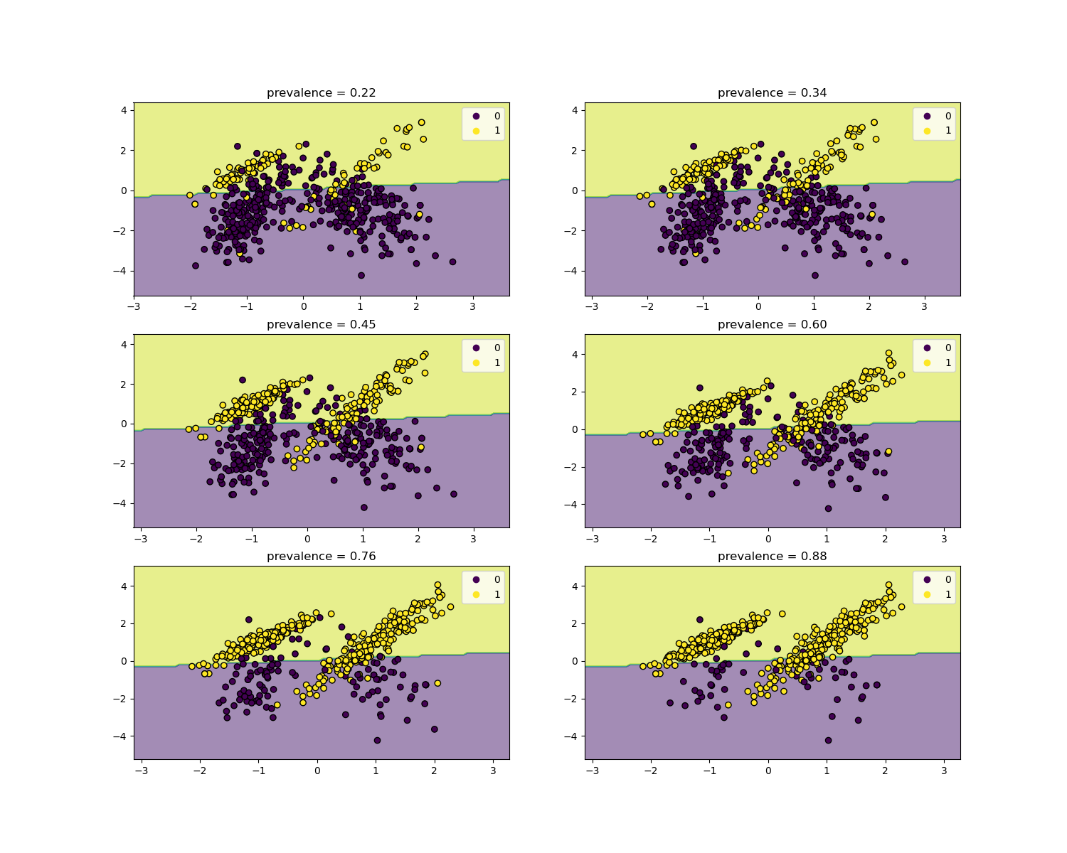
Invariance with respect to prevalence#
The likelihood ratios are independent of the disease prevalence and can be extrapolated between populations regardless of any possible class imbalance, as long as the same model is applied to all of them. Notice that in the plots below the decision boundary is constant (see SVM: Separating hyperplane for unbalanced classes for a study of the boundary decision for unbalanced classes).
Here we train a LogisticRegression base model
on a case-control study with a prevalence of 50%. It is then evaluated over
populations with varying prevalence. We use the
make_classification function to ensure the
data-generating process is always the same as shown in the plots below. The
label 1 corresponds to the positive class “disease”, whereas the label 0
stands for “no-disease”.
from collections import defaultdict

import matplotlib.pyplot as plt
import numpy as np

from sklearn.inspection import DecisionBoundaryDisplay

populations = defaultdict(list)
common_params = {
    "n_samples": 10_000,
    "n_features": 2,
    "n_informative": 2,
    "n_redundant": 0,
    "random_state": 0,
}
weights = np.linspace(0.1, 0.8, 6)
weights = weights[::-1]

# fit and evaluate base model on balanced classes
X, y = make_classification(**common_params, weights=[0.5, 0.5])
estimator = LogisticRegression().fit(X, y)
lr_base = extract_score(cross_validate(estimator, X, y, scoring=scoring, cv=10))
pos_lr_base, pos_lr_base_std = lr_base["positive"].values
neg_lr_base, neg_lr_base_std = lr_base["negative"].values
We will now show the decision boundary for each level of prevalence. Note that we only plot a subset of the original data to better assess the linear model decision boundary.
fig, axs = plt.subplots(nrows=3, ncols=2, figsize=(15, 12))

for ax, (n, weight) in zip(axs.ravel(), enumerate(weights)):
    X, y = make_classification(
        **common_params,
        weights=[weight, 1 - weight],
    )
    prevalence = y.mean()
    populations["prevalence"].append(prevalence)
    populations["X"].append(X)
    populations["y"].append(y)

    # down-sample for plotting
    rng = np.random.RandomState(1)
    plot_indices = rng.choice(np.arange(X.shape[0]), size=500, replace=True)
    X_plot, y_plot = X[plot_indices], y[plot_indices]

    # plot fixed decision boundary of base model with varying prevalence
    disp = DecisionBoundaryDisplay.from_estimator(
        estimator,
        X_plot,
        response_method="predict",
        alpha=0.5,
        ax=ax,
    )
    scatter = disp.ax_.scatter(X_plot[:, 0], X_plot[:, 1], c=y_plot, edgecolor="k")
    disp.ax_.set_title(f"prevalence = {y_plot.mean():.2f}")
    disp.ax_.legend(*scatter.legend_elements())
We define a function for bootstrapping.
def scoring_on_bootstrap(estimator, X, y, rng, n_bootstrap=100):
    results_for_prevalence = defaultdict(list)
    for _ in range(n_bootstrap):
        bootstrap_indices = rng.choice(
            np.arange(X.shape[0]), size=X.shape[0], replace=True
        )
        for key, value in scoring(
            estimator, X[bootstrap_indices], y[bootstrap_indices]
        ).items():
            results_for_prevalence[key].append(value)
    return pd.DataFrame(results_for_prevalence)
We score the base model for each prevalence using bootstrapping.
results = defaultdict(list)
n_bootstrap = 100
rng = np.random.default_rng(seed=0)

for prevalence, X, y in zip(
    populations["prevalence"], populations["X"], populations["y"]
):
    results_for_prevalence = scoring_on_bootstrap(
        estimator, X, y, rng, n_bootstrap=n_bootstrap
    )
    results["prevalence"].append(prevalence)
    results["metrics"].append(
        results_for_prevalence.aggregate(["mean", "std"]).unstack()
    )

results = pd.DataFrame(results["metrics"], index=results["prevalence"])
results.index.name = "prevalence"
results
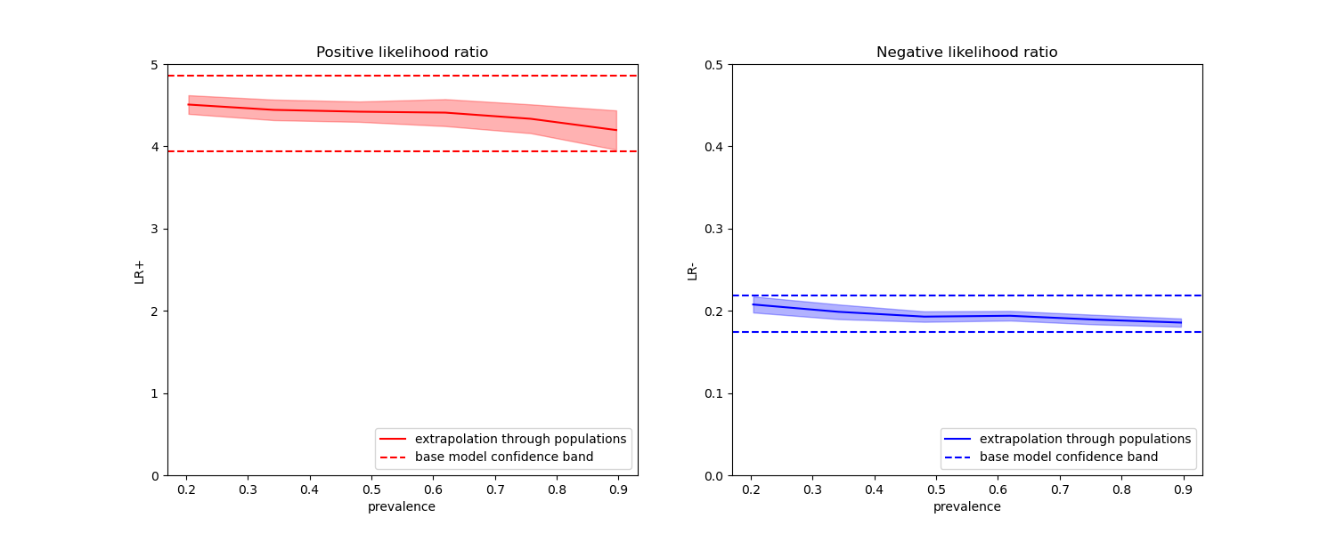
In the plots below we observe that the class likelihood ratios re-computed with different prevalences are indeed constant within one standard deviation of those computed with on balanced classes.
fig, (ax1, ax2) = plt.subplots(nrows=1, ncols=2, figsize=(15, 6))
results["positive_likelihood_ratio"]["mean"].plot(
    ax=ax1, color="r", label="extrapolation through populations"
)
ax1.axhline(y=pos_lr_base + pos_lr_base_std, color="r", linestyle="--")
ax1.axhline(
    y=pos_lr_base - pos_lr_base_std,
    color="r",
    linestyle="--",
    label="base model confidence band",
)
ax1.fill_between(
    results.index,
    results["positive_likelihood_ratio"]["mean"]
    - results["positive_likelihood_ratio"]["std"],
    results["positive_likelihood_ratio"]["mean"]
    + results["positive_likelihood_ratio"]["std"],
    color="r",
    alpha=0.3,
)
ax1.set(
    title="Positive likelihood ratio",
    ylabel="LR+",
    ylim=[0, 5],
)
ax1.legend(loc="lower right")

ax2 = results["negative_likelihood_ratio"]["mean"].plot(
    ax=ax2, color="b", label="extrapolation through populations"
)
ax2.axhline(y=neg_lr_base + neg_lr_base_std, color="b", linestyle="--")
ax2.axhline(
    y=neg_lr_base - neg_lr_base_std,
    color="b",
    linestyle="--",
    label="base model confidence band",
)
ax2.fill_between(
    results.index,
    results["negative_likelihood_ratio"]["mean"]
    - results["negative_likelihood_ratio"]["std"],
    results["negative_likelihood_ratio"]["mean"]
    + results["negative_likelihood_ratio"]["std"],
    color="b",
    alpha=0.3,
)
ax2.set(
    title="Negative likelihood ratio",
    ylabel="LR-",
    ylim=[0, 0.5],
)
ax2.legend(loc="lower right")

plt.show()
Total running time of the script: (0 minutes 3.692 seconds)
Related examples
Post-hoc tuning the cut-off point of decision function