Note
Go to the end to download the full example code or to run this example in your browser via JupyterLite or Binder.
Shrinkage covariance estimation: LedoitWolf vs OAS and max-likelihood#
When working with covariance estimation, the usual approach is to use
a maximum likelihood estimator, such as the
EmpiricalCovariance. It is unbiased, i.e. it
converges to the true (population) covariance when given many
observations. However, it can also be beneficial to regularize it, in
order to reduce its variance; this, in turn, introduces some bias. This
example illustrates the simple regularization used in
Shrunk Covariance estimators. In particular, it focuses on how to
set the amount of regularization, i.e. how to choose the bias-variance
trade-off.
References
# Authors: The scikit-learn developers
# SPDX-License-Identifier: BSD-3-Clause
Generate sample data#
import numpy as np

n_features, n_samples = 40, 20
np.random.seed(42)
base_X_train = np.random.normal(size=(n_samples, n_features))
base_X_test = np.random.normal(size=(n_samples, n_features))

# Color samples
coloring_matrix = np.random.normal(size=(n_features, n_features))
X_train = np.dot(base_X_train, coloring_matrix)
X_test = np.dot(base_X_test, coloring_matrix)
Compute the likelihood on test data#
from scipy import linalg

from sklearn.covariance import ShrunkCovariance, empirical_covariance, log_likelihood

# spanning a range of possible shrinkage coefficient values
shrinkages = np.logspace(-2, 0, 30)
negative_logliks = [
    -ShrunkCovariance(shrinkage=s).fit(X_train).score(X_test) for s in shrinkages
]

# under the ground-truth model, which we would not have access to in real
# settings
real_cov = np.dot(coloring_matrix.T, coloring_matrix)
emp_cov = empirical_covariance(X_train)
loglik_real = -log_likelihood(emp_cov, linalg.inv(real_cov))
Compare different approaches to setting the regularization parameter#
Here we compare 3 approaches:
Setting the parameter by cross-validating the likelihood on three folds according to a grid of potential shrinkage parameters.
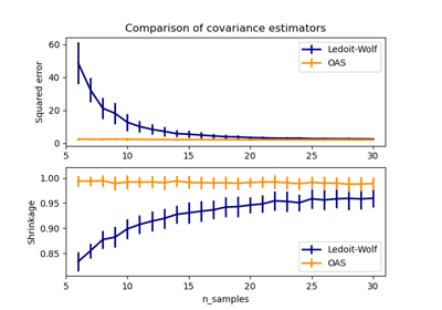
A close formula proposed by Ledoit and Wolf to compute the asymptotically optimal regularization parameter (minimizing an MSE criterion), yielding the
LedoitWolfcovariance estimate.An improvement of the Ledoit-Wolf shrinkage, the
OAS, proposed by Chen et al. [1]. Its convergence is significantly better under the assumption that the data are Gaussian, in particular for small samples.
from sklearn.covariance import OAS, LedoitWolf
from sklearn.model_selection import GridSearchCV

# GridSearch for an optimal shrinkage coefficient
tuned_parameters = [{"shrinkage": shrinkages}]
cv = GridSearchCV(ShrunkCovariance(), tuned_parameters)
cv.fit(X_train)

# Ledoit-Wolf optimal shrinkage coefficient estimate
lw = LedoitWolf()
loglik_lw = lw.fit(X_train).score(X_test)

# OAS coefficient estimate
oa = OAS()
loglik_oa = oa.fit(X_train).score(X_test)
Plot results#
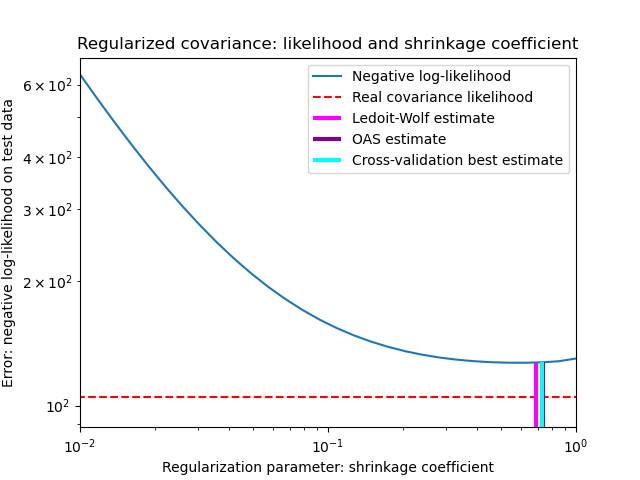
To quantify estimation error, we plot the likelihood of unseen data for different values of the shrinkage parameter. We also show the choices by cross-validation, or with the LedoitWolf and OAS estimates.
import matplotlib.pyplot as plt

fig = plt.figure()
plt.title("Regularized covariance: likelihood and shrinkage coefficient")
plt.xlabel("Regularization parameter: shrinkage coefficient")
plt.ylabel("Error: negative log-likelihood on test data")
# range shrinkage curve
plt.loglog(shrinkages, negative_logliks, label="Negative log-likelihood")

plt.plot(plt.xlim(), 2 * [loglik_real], "--r", label="Real covariance likelihood")

# adjust view
lik_max = np.amax(negative_logliks)
lik_min = np.amin(negative_logliks)
ymin = lik_min - 6.0 * np.log((plt.ylim()[1] - plt.ylim()[0]))
ymax = lik_max + 10.0 * np.log(lik_max - lik_min)
xmin = shrinkages[0]
xmax = shrinkages[-1]
# LW likelihood
plt.vlines(
    lw.shrinkage_,
    ymin,
    -loglik_lw,
    color="magenta",
    linewidth=3,
    label="Ledoit-Wolf estimate",
)
# OAS likelihood
plt.vlines(
    oa.shrinkage_, ymin, -loglik_oa, color="purple", linewidth=3, label="OAS estimate"
)
# best CV estimator likelihood
plt.vlines(
    cv.best_estimator_.shrinkage,
    ymin,
    -cv.best_estimator_.score(X_test),
    color="cyan",
    linewidth=3,
    label="Cross-validation best estimate",
)

plt.ylim(ymin, ymax)
plt.xlim(xmin, xmax)
plt.legend()

plt.show()
Note
The maximum likelihood estimate corresponds to no shrinkage, and thus performs poorly. The Ledoit-Wolf estimate performs really well, as it is close to the optimal and is not computationally costly. In this example, the OAS estimate is a bit further away. Interestingly, both approaches outperform cross-validation, which is significantly most computationally costly.
Total running time of the script: (0 minutes 0.532 seconds)
Related examples
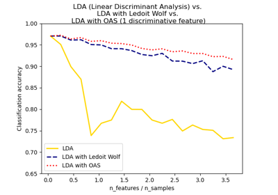
Normal, Ledoit-Wolf and OAS Linear Discriminant Analysis for classification