Note
Go to the end to download the full example code or to run this example in your browser via JupyterLite or Binder.
The Johnson-Lindenstrauss bound for embedding with random projections#
The Johnson-Lindenstrauss lemma states that any high dimensional dataset can be randomly projected into a lower dimensional Euclidean space while controlling the distortion in the pairwise distances.
# Authors: The scikit-learn developers
# SPDX-License-Identifier: BSD-3-Clause

import sys
from time import time

import matplotlib.pyplot as plt
import numpy as np

from sklearn.datasets import fetch_20newsgroups_vectorized, load_digits
from sklearn.metrics.pairwise import euclidean_distances
from sklearn.random_projection import (
    SparseRandomProjection,
    johnson_lindenstrauss_min_dim,
)
Theoretical bounds#
The distortion introduced by a random projection p is asserted by
the fact that p is defining an eps-embedding with good probability
as defined by:
Where u and v are any rows taken from a dataset of shape (n_samples,
n_features) and p is a projection by a random Gaussian N(0, 1) matrix
of shape (n_components, n_features) (or a sparse Achlioptas matrix).
The minimum number of components to guarantees the eps-embedding is given by:
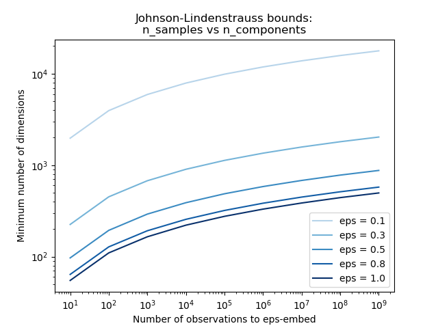
The first plot shows that with an increasing number of samples n_samples,
the minimal number of dimensions n_components increased logarithmically
in order to guarantee an eps-embedding.
# range of admissible distortions
eps_range = np.linspace(0.1, 0.99, 5)
colors = plt.cm.Blues(np.linspace(0.3, 1.0, len(eps_range)))

# range of number of samples (observation) to embed
n_samples_range = np.logspace(1, 9, 9)

plt.figure()
for eps, color in zip(eps_range, colors):
    min_n_components = johnson_lindenstrauss_min_dim(n_samples_range, eps=eps)
    plt.loglog(n_samples_range, min_n_components, color=color)

plt.legend([f"eps = {eps:0.1f}" for eps in eps_range], loc="lower right")
plt.xlabel("Number of observations to eps-embed")
plt.ylabel("Minimum number of dimensions")
plt.title("Johnson-Lindenstrauss bounds:\nn_samples vs n_components")
plt.show()
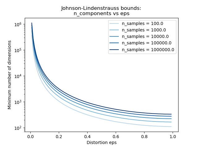
The second plot shows that an increase of the admissible
distortion eps allows to reduce drastically the minimal number of
dimensions n_components for a given number of samples n_samples
# range of admissible distortions
eps_range = np.linspace(0.01, 0.99, 100)

# range of number of samples (observation) to embed
n_samples_range = np.logspace(2, 6, 5)
colors = plt.cm.Blues(np.linspace(0.3, 1.0, len(n_samples_range)))

plt.figure()
for n_samples, color in zip(n_samples_range, colors):
    min_n_components = johnson_lindenstrauss_min_dim(n_samples, eps=eps_range)
    plt.semilogy(eps_range, min_n_components, color=color)

plt.legend([f"n_samples = {n}" for n in n_samples_range], loc="upper right")
plt.xlabel("Distortion eps")
plt.ylabel("Minimum number of dimensions")
plt.title("Johnson-Lindenstrauss bounds:\nn_components vs eps")
plt.show()
Empirical validation#
We validate the above bounds on the 20 newsgroups text document (TF-IDF word frequencies) dataset or on the digits dataset:
for the 20 newsgroups dataset some 300 documents with 100k features in total are projected using a sparse random matrix to smaller euclidean spaces with various values for the target number of dimensions
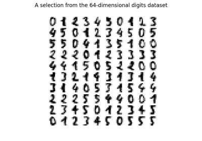
n_components.for the digits dataset, some 8x8 gray level pixels data for 300 handwritten digits pictures are randomly projected to spaces for various larger number of dimensions
n_components.
The default dataset is the 20 newsgroups dataset. To run the example on the
digits dataset, pass the --use-digits-dataset command line argument to
this script.
if "--use-digits-dataset" in sys.argv:
    data = load_digits().data[:300]
else:
    data = fetch_20newsgroups_vectorized().data[:300]
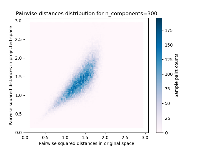
For each value of n_components, we plot:
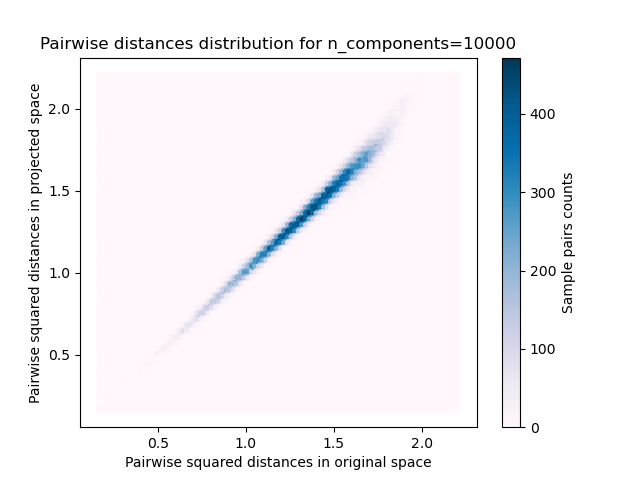
2D distribution of sample pairs with pairwise distances in original and projected spaces as x- and y-axis respectively.
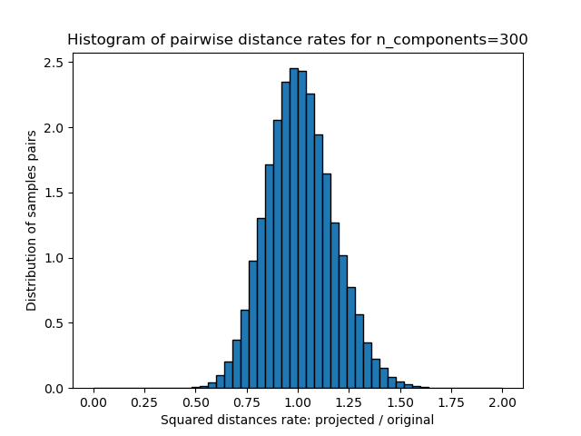
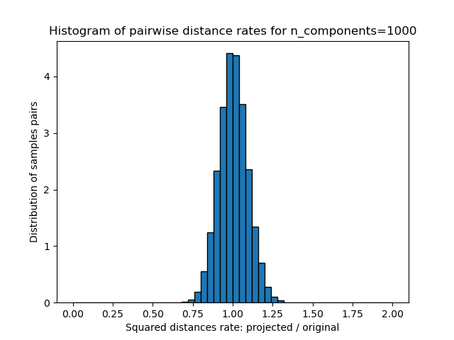
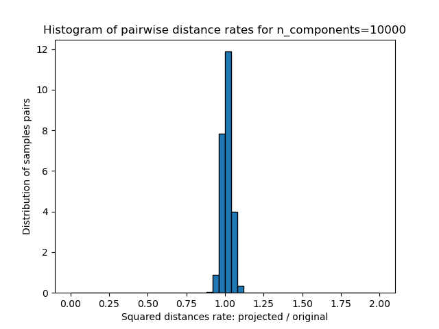
1D histogram of the ratio of those distances (projected / original).
n_samples, n_features = data.shape
print(
    f"Embedding {n_samples} samples with dim {n_features} using various "
    "random projections"
)

n_components_range = np.array([300, 1_000, 10_000])
dists = euclidean_distances(data, squared=True).ravel()

# select only non-identical samples pairs
nonzero = dists != 0
dists = dists[nonzero]

for n_components in n_components_range:
    t0 = time()
    rp = SparseRandomProjection(n_components=n_components)
    projected_data = rp.fit_transform(data)
    print(
        f"Projected {n_samples} samples from {n_features} to {n_components} in "
        f"{time() - t0:0.3f}s"
    )
    if hasattr(rp, "components_"):
        n_bytes = rp.components_.data.nbytes
        n_bytes += rp.components_.indices.nbytes
        print(f"Random matrix with size: {n_bytes / 1e6:0.3f} MB")

    projected_dists = euclidean_distances(projected_data, squared=True).ravel()[nonzero]

    plt.figure()
    min_dist = min(projected_dists.min(), dists.min())
    max_dist = max(projected_dists.max(), dists.max())
    plt.hexbin(
        dists,
        projected_dists,
        gridsize=100,
        cmap=plt.cm.PuBu,
        extent=[min_dist, max_dist, min_dist, max_dist],
    )
    plt.xlabel("Pairwise squared distances in original space")
    plt.ylabel("Pairwise squared distances in projected space")
    plt.title("Pairwise distances distribution for n_components=%d" % n_components)
    cb = plt.colorbar()
    cb.set_label("Sample pairs counts")

    rates = projected_dists / dists
    print(f"Mean distances rate: {np.mean(rates):.2f} ({np.std(rates):.2f})")

    plt.figure()
    plt.hist(rates, bins=50, range=(0.0, 2.0), edgecolor="k", density=True)
    plt.xlabel("Squared distances rate: projected / original")
    plt.ylabel("Distribution of samples pairs")
    plt.title("Histogram of pairwise distance rates for n_components=%d" % n_components)

    # TODO: compute the expected value of eps and add them to the previous plot
    # as vertical lines / region

plt.show()
Embedding 300 samples with dim 130107 using various random projections
Projected 300 samples from 130107 to 300 in 0.262s
Random matrix with size: 1.293 MB
Mean distances rate: 1.01 (0.16)
Projected 300 samples from 130107 to 1000 in 0.850s
Random matrix with size: 4.333 MB
Mean distances rate: 1.00 (0.09)
Projected 300 samples from 130107 to 10000 in 7.971s
Random matrix with size: 43.239 MB
Mean distances rate: 1.01 (0.03)
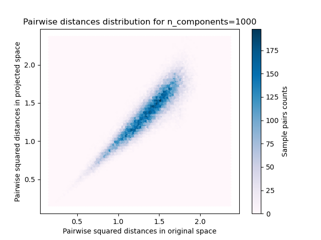
We can see that for low values of n_components the distribution is wide
with many distorted pairs and a skewed distribution (due to the hard
limit of zero ratio on the left as distances are always positives)
while for larger values of n_components the distortion is controlled
and the distances are well preserved by the random projection.
Remarks#
According to the JL lemma, projecting 300 samples without too much distortion will require at least several thousands dimensions, irrespective of the number of features of the original dataset.
Hence using random projections on the digits dataset which only has 64 features in the input space does not make sense: it does not allow for dimensionality reduction in this case.
On the twenty newsgroups on the other hand the dimensionality can be decreased from 56,436 down to 10,000 while reasonably preserving pairwise distances.
Total running time of the script: (0 minutes 11.304 seconds)
Related examples
Manifold learning on handwritten digits: Locally Linear Embedding, Isomap…