Note
Go to the end to download the full example code or to run this example in your browser via JupyterLite or Binder.
Failure of Machine Learning to infer causal effects#
Machine Learning models are great for measuring statistical associations. Unfortunately, unless we’re willing to make strong assumptions about the data, those models are unable to infer causal effects.
To illustrate this, we will simulate a situation in which we try to answer one of the most important questions in economics of education: what is the causal effect of earning a college degree on hourly wages? Although the answer to this question is crucial to policy makers, Omitted-Variable Biases (OVB) prevent us from identifying that causal effect.
# Authors: The scikit-learn developers
# SPDX-License-Identifier: BSD-3-Clause
The dataset: simulated hourly wages#
The data generating process is laid out in the code below. Work experience in years and a measure of ability are drawn from Normal distributions; the hourly wage of one of the parents is drawn from Beta distribution. We then create an indicator of college degree which is positively impacted by ability and parental hourly wage. Finally, we model hourly wages as a linear function of all the previous variables and a random component. Note that all variables have a positive effect on hourly wages.
import numpy as np
import pandas as pd

n_samples = 10_000
rng = np.random.RandomState(32)

experiences = rng.normal(20, 10, size=n_samples).astype(int)
experiences[experiences < 0] = 0
abilities = rng.normal(0, 0.15, size=n_samples)
parent_hourly_wages = 50 * rng.beta(2, 8, size=n_samples)
parent_hourly_wages[parent_hourly_wages < 0] = 0
college_degrees = (
    9 * abilities + 0.02 * parent_hourly_wages + rng.randn(n_samples) > 0.7
).astype(int)

true_coef = pd.Series(
    {
        "college degree": 2.0,
        "ability": 5.0,
        "experience": 0.2,
        "parent hourly wage": 1.0,
    }
)
hourly_wages = (
    true_coef["experience"] * experiences
    + true_coef["parent hourly wage"] * parent_hourly_wages
    + true_coef["college degree"] * college_degrees
    + true_coef["ability"] * abilities
    + rng.normal(0, 1, size=n_samples)
)

hourly_wages[hourly_wages < 0] = 0
Description of the simulated data#
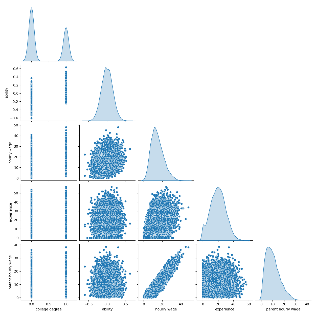
The following plot shows the distribution of each variable, and pairwise scatter plots. Key to our OVB story is the positive relationship between ability and college degree.
import seaborn as sns

df = pd.DataFrame(
    {
        "college degree": college_degrees,
        "ability": abilities,
        "hourly wage": hourly_wages,
        "experience": experiences,
        "parent hourly wage": parent_hourly_wages,
    }
)

grid = sns.pairplot(df, diag_kind="kde", corner=True)
In the next section, we train predictive models and we therefore split the target column from over features and we split the data into a training and a testing set.
from sklearn.model_selection import train_test_split

target_name = "hourly wage"
X, y = df.drop(columns=target_name), df[target_name]
X_train, X_test, y_train, y_test = train_test_split(X, y, test_size=0.2, random_state=0)
Income prediction with fully observed variables#
First, we train a predictive model, a
LinearRegression model. In this experiment,
we assume that all variables used by the true generative model are available.
from sklearn.linear_model import LinearRegression
from sklearn.metrics import r2_score

features_names = ["experience", "parent hourly wage", "college degree", "ability"]

regressor_with_ability = LinearRegression()
regressor_with_ability.fit(X_train[features_names], y_train)
y_pred_with_ability = regressor_with_ability.predict(X_test[features_names])
R2_with_ability = r2_score(y_test, y_pred_with_ability)

print(f"R2 score with ability: {R2_with_ability:.3f}")
R2 score with ability: 0.975
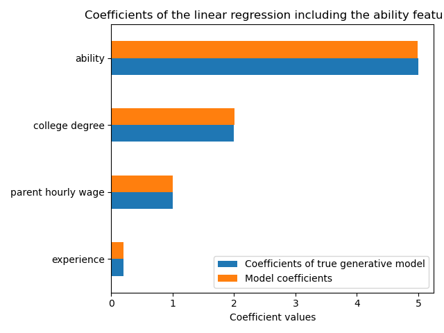
This model predicts well the hourly wages as shown by the high R2 score. We plot the model coefficients to show that we exactly recover the values of the true generative model.
import matplotlib.pyplot as plt

model_coef = pd.Series(regressor_with_ability.coef_, index=features_names)
coef = pd.concat(
    [true_coef[features_names], model_coef],
    keys=["Coefficients of true generative model", "Model coefficients"],
    axis=1,
)
ax = coef.plot.barh()
ax.set_xlabel("Coefficient values")
ax.set_title("Coefficients of the linear regression including the ability features")
_ = plt.tight_layout()
Income prediction with partial observations#
In practice, intellectual abilities are not observed or are only estimated from proxies that inadvertently measure education as well (e.g. by IQ tests). But omitting the “ability” feature from a linear model inflates the estimate via a positive OVB.
features_names = ["experience", "parent hourly wage", "college degree"]

regressor_without_ability = LinearRegression()
regressor_without_ability.fit(X_train[features_names], y_train)
y_pred_without_ability = regressor_without_ability.predict(X_test[features_names])
R2_without_ability = r2_score(y_test, y_pred_without_ability)

print(f"R2 score without ability: {R2_without_ability:.3f}")
R2 score without ability: 0.968
The predictive power of our model is similar when we omit the ability feature in terms of R2 score. We now check if the coefficient of the model are different from the true generative model.
model_coef = pd.Series(regressor_without_ability.coef_, index=features_names)
coef = pd.concat(
    [true_coef[features_names], model_coef],
    keys=["Coefficients of true generative model", "Model coefficients"],
    axis=1,
)
ax = coef.plot.barh()
ax.set_xlabel("Coefficient values")
_ = ax.set_title("Coefficients of the linear regression excluding the ability feature")
plt.tight_layout()
plt.show()
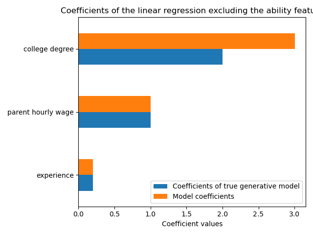
To compensate for the omitted variable, the model inflates the coefficient of the college degree feature. Therefore, interpreting this coefficient value as a causal effect of the true generative model is incorrect.
Lessons learned#
Machine learning models are not designed for the estimation of causal effects. While we showed this with a linear model, OVB can affect any type of model.
Whenever interpreting a coefficient or a change in predictions brought about by a change in one of the features, it is important to keep in mind potentially unobserved variables that could be correlated with both the feature in question and the target variable. Such variables are called Confounding Variables. In order to still estimate causal effect in the presence of confounding, researchers usually conduct experiments in which the treatment variable (e.g. college degree) is randomized. When an experiment is prohibitively expensive or unethical, researchers can sometimes use other causal inference techniques such as Instrumental Variables (IV) estimations.
Total running time of the script: (0 minutes 2.129 seconds)
Related examples
Common pitfalls in the interpretation of coefficients of linear models
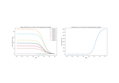
Ridge coefficients as a function of the L2 Regularization
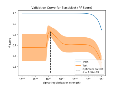
Effect of model regularization on training and test error
