Note

Go to the end to download the full example code or to run this example in your browser via JupyterLite or Binder

Pipeline ANOVA SVM¶

This example shows how a feature selection can be easily integrated within a machine learning pipeline.

We also show that you can easily inspect part of the pipeline.

We will start by generating a binary classification dataset. Subsequently, we will divide the dataset into two subsets.

from sklearn.datasets import make_classification
from sklearn.model_selection import train_test_split

X, y = make_classification(
    n_features=20,
    n_informative=3,
    n_redundant=0,
    n_classes=2,
    n_clusters_per_class=2,
    random_state=42,
)
X_train, X_test, y_train, y_test = train_test_split(X, y, random_state=42)

A common mistake done with feature selection is to search a subset of discriminative features on the full dataset, instead of only using the training set. The usage of scikit-learn Pipeline prevents to make such mistake.

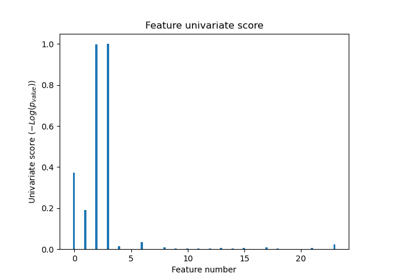
Here, we will demonstrate how to build a pipeline where the first step will be the feature selection.

When calling fit on the training data, a subset of feature will be selected and the index of these selected features will be stored. The feature selector will subsequently reduce the number of features, and pass this subset to the classifier which will be trained.

from sklearn.feature_selection import SelectKBest, f_classif
from sklearn.pipeline import make_pipeline
from sklearn.svm import LinearSVC

anova_filter = SelectKBest(f_classif, k=3)
clf = LinearSVC(dual="auto")
anova_svm = make_pipeline(anova_filter, clf)
anova_svm.fit(X_train, y_train)

Pipeline(steps=[('selectkbest', SelectKBest(k=3)),
                ('linearsvc', LinearSVC(dual='auto'))])

In a Jupyter environment, please rerun this cell to show the HTML representation or trust the notebook.
On GitHub, the HTML representation is unable to render, please try loading this page with nbviewer.org.

Once the training is complete, we can predict on new unseen samples. In this case, the feature selector will only select the most discriminative features based on the information stored during training. Then, the data will be passed to the classifier which will make the prediction.

Here, we show the final metrics via a classification report.

from sklearn.metrics import classification_report

y_pred = anova_svm.predict(X_test)
print(classification_report(y_test, y_pred))

              precision    recall  f1-score   support

           0       0.92      0.80      0.86        15
           1       0.75      0.90      0.82        10

    accuracy                           0.84        25
   macro avg       0.84      0.85      0.84        25
weighted avg       0.85      0.84      0.84        25

Be aware that you can inspect a step in the pipeline. For instance, we might be interested about the parameters of the classifier. Since we selected three features, we expect to have three coefficients.

anova_svm[-1].coef_

array([[0.75788833, 0.27161955, 0.26113448]])

However, we do not know which features were selected from the original dataset. We could proceed by several manners. Here, we will invert the transformation of these coefficients to get information about the original space.

anova_svm[:-1].inverse_transform(anova_svm[-1].coef_)

array([[0.        , 0.        , 0.75788833, 0.        , 0.        ,
        0.        , 0.        , 0.        , 0.        , 0.27161955,
        0.        , 0.        , 0.        , 0.        , 0.        ,
        0.        , 0.        , 0.        , 0.        , 0.26113448]])

We can see that the features with non-zero coefficients are the selected features by the first step.

Total running time of the script: (0 minutes 0.013 seconds)