Note
Go to the end to download the full example code or to run this example in your browser via JupyterLite or Binder.
Nearest Neighbors Classification#
This example shows how to use KNeighborsClassifier.
We train such a classifier on the iris dataset and observe the difference of the
decision boundary obtained with regards to the parameter weights.
# Authors: The scikit-learn developers
# SPDX-License-Identifier: BSD-3-Clause
Load the data#
In this example, we use the iris dataset. We split the data into a train and test dataset.
from sklearn.datasets import load_iris
from sklearn.model_selection import train_test_split

iris = load_iris(as_frame=True)
X = iris.data[["sepal length (cm)", "sepal width (cm)"]]
y = iris.target
X_train, X_test, y_train, y_test = train_test_split(X, y, stratify=y, random_state=0)
K-nearest neighbors classifier#
We want to use a k-nearest neighbors classifier considering a neighborhood of 11 data points. Since our k-nearest neighbors model uses euclidean distance to find the nearest neighbors, it is therefore important to scale the data beforehand. Refer to the example entitled Importance of Feature Scaling for more detailed information.
Thus, we use a Pipeline to chain a scaler before to use
our classifier.
from sklearn.neighbors import KNeighborsClassifier
from sklearn.pipeline import Pipeline
from sklearn.preprocessing import StandardScaler

clf = Pipeline(
    steps=[("scaler", StandardScaler()), ("knn", KNeighborsClassifier(n_neighbors=11))]
)
Decision boundary#
Now, we fit two classifiers with different values of the parameter
weights. We plot the decision boundary of each classifier as well as the original
dataset to observe the difference.
import matplotlib as mpl
import matplotlib.pyplot as plt

from sklearn.inspection import DecisionBoundaryDisplay

_, axs = plt.subplots(ncols=2, figsize=(12, 5))

for ax, weights in zip(axs, ("uniform", "distance")):
    clf.set_params(knn__weights=weights).fit(X_train, y_train)
    disp = DecisionBoundaryDisplay.from_estimator(
        clf,
        X_test,
        response_method="predict",
        plot_method="pcolormesh",
        xlabel=iris.feature_names[0],
        ylabel=iris.feature_names[1],
        shading="auto",
        alpha=0.5,
        ax=ax,
    )
    cmap = mpl.colors.ListedColormap(disp.multiclass_colors_)
    scatter = disp.ax_.scatter(
        X.iloc[:, 0], X.iloc[:, 1], c=y, cmap=cmap, edgecolors="k"
    )
    disp.ax_.legend(
        scatter.legend_elements()[0],
        iris.target_names,
        loc="lower right",
        title="Classes",
    )
    _ = disp.ax_.set_title(
        f"3-Class classification\n(k={clf[-1].n_neighbors}, weights={weights!r})"
    )

plt.show()
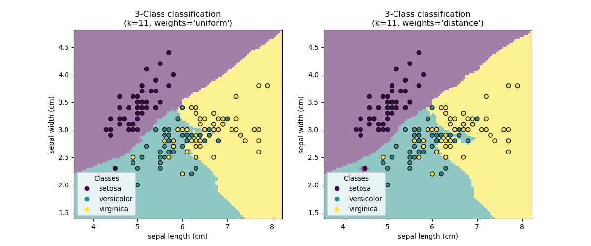
Conclusion#
We observe that the parameter weights has an impact on the decision boundary. When
weights="uniform" all nearest neighbors will have the same impact on the decision.
Whereas when weights="distance" the weight given to each neighbor is proportional
to the inverse of the distance from that neighbor to the query point.
In some cases, taking the distance into account might improve the model.
Total running time of the script: (0 minutes 0.221 seconds)
Related examples
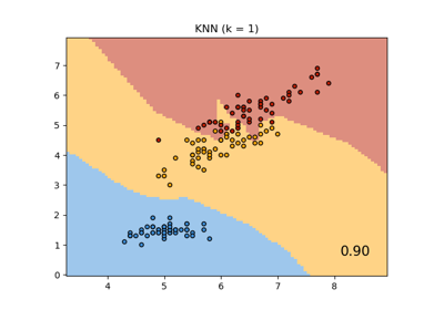
Comparing Nearest Neighbors with and without Neighborhood Components Analysis
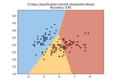
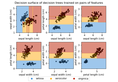
Plot the decision surface of decision trees trained on the iris dataset
