Note
Go to the end to download the full example code or to run this example in your browser via JupyterLite or Binder.
Imputing missing values with variants of IterativeImputer#
The IterativeImputer class is very flexible - it can be
used with a variety of estimators to do round-robin regression, treating every
variable as an output in turn.
In this example we compare some estimators for the purpose of missing feature
imputation with IterativeImputer:
BayesianRidge: regularized linear regressionRandomForestRegressor: forests of randomized trees regressionmake_pipeline(Nystroem,Ridge): a pipeline with the expansion of a degree 2 polynomial kernel and regularized linear regressionKNeighborsRegressor: comparable to other KNN imputation approaches
Of particular interest is the ability of
IterativeImputer to mimic the behavior of missForest, a
popular imputation package for R.
Note that KNeighborsRegressor is different from KNN
imputation, which learns from samples with missing values by using a distance
metric that accounts for missing values, rather than imputing them.
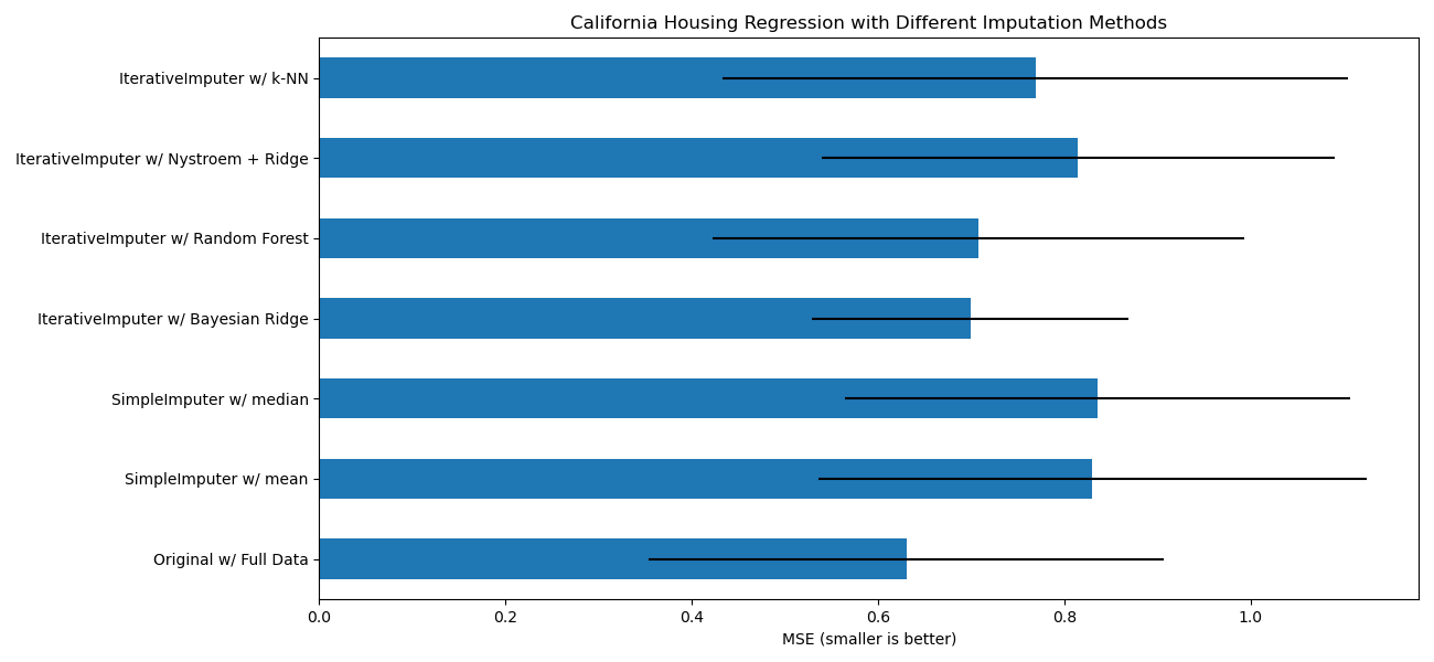
The goal is to compare different estimators to see which one is best for the
IterativeImputer when using a
BayesianRidge estimator on the California housing
dataset with a single value randomly removed from each row.
For this particular pattern of missing values we see that
BayesianRidge and
RandomForestRegressor give the best results.
It should be noted that some estimators such as
HistGradientBoostingRegressor can natively deal with
missing features and are often recommended over building pipelines with
complex and costly missing values imputation strategies.
# Authors: The scikit-learn developers
# SPDX-License-Identifier: BSD-3-Clause

import matplotlib.pyplot as plt
import numpy as np
import pandas as pd

from sklearn.datasets import fetch_california_housing
from sklearn.ensemble import RandomForestRegressor

# To use this experimental feature, we need to explicitly ask for it:
from sklearn.experimental import enable_iterative_imputer  # noqa: F401
from sklearn.impute import IterativeImputer, SimpleImputer
from sklearn.kernel_approximation import Nystroem
from sklearn.linear_model import BayesianRidge, Ridge
from sklearn.model_selection import cross_val_score
from sklearn.neighbors import KNeighborsRegressor
from sklearn.pipeline import make_pipeline
from sklearn.preprocessing import RobustScaler

N_SPLITS = 5

X_full, y_full = fetch_california_housing(return_X_y=True)
# ~2k samples is enough for the purpose of the example.
# Remove the following two lines for a slower run with different error bars.
X_full = X_full[::10]
y_full = y_full[::10]
n_samples, n_features = X_full.shape


def compute_score_for(X, y, imputer=None):
    # We scale data before imputation and training a target estimator,
    # because our target estimator and some of the imputers assume
    # that the features have similar scales.
    if imputer is None:
        estimator = make_pipeline(RobustScaler(), BayesianRidge())
    else:
        estimator = make_pipeline(RobustScaler(), imputer, BayesianRidge())
    return cross_val_score(
        estimator, X, y, scoring="neg_mean_squared_error", cv=N_SPLITS
    )


# Estimate the score on the entire dataset, with no missing values
score_full_data = pd.DataFrame(
    compute_score_for(X_full, y_full),
    columns=["Full Data"],
)

# Add a single missing value to each row
rng = np.random.RandomState(0)
X_missing = X_full.copy()
y_missing = y_full
missing_samples = np.arange(n_samples)
missing_features = rng.choice(n_features, n_samples, replace=True)
X_missing[missing_samples, missing_features] = np.nan

# Estimate the score after imputation (mean and median strategies)
score_simple_imputer = pd.DataFrame()
for strategy in ("mean", "median"):
    score_simple_imputer[strategy] = compute_score_for(
        X_missing, y_missing, SimpleImputer(strategy=strategy)
    )

# Estimate the score after iterative imputation of the missing values
# with different estimators
named_estimators = [
    ("Bayesian Ridge", BayesianRidge()),
    (
        "Random Forest",
        RandomForestRegressor(
            # We tuned the hyperparameters of the RandomForestRegressor to get a good
            # enough predictive performance for a restricted execution time.
            n_estimators=5,
            max_depth=10,
            bootstrap=True,
            max_samples=0.5,
            n_jobs=2,
            random_state=0,
        ),
    ),
    (
        "Nystroem + Ridge",
        make_pipeline(
            Nystroem(kernel="polynomial", degree=2, random_state=0), Ridge(alpha=1e4)
        ),
    ),
    (
        "k-NN",
        KNeighborsRegressor(n_neighbors=10),
    ),
]
score_iterative_imputer = pd.DataFrame()
# Iterative imputer is sensitive to the tolerance and
# dependent on the estimator used internally.
# We tuned the tolerance to keep this example run with limited computational
# resources while not changing the results too much compared to keeping the
# stricter default value for the tolerance parameter.
tolerances = (1e-3, 1e-1, 1e-1, 1e-2)
for (name, impute_estimator), tol in zip(named_estimators, tolerances):
    score_iterative_imputer[name] = compute_score_for(
        X_missing,
        y_missing,
        IterativeImputer(
            random_state=0, estimator=impute_estimator, max_iter=40, tol=tol
        ),
    )

scores = pd.concat(
    [score_full_data, score_simple_imputer, score_iterative_imputer],
    keys=["Original", "SimpleImputer", "IterativeImputer"],
    axis=1,
)

# plot california housing results
fig, ax = plt.subplots(figsize=(13, 6))
means = -scores.mean()
errors = scores.std()
means.plot.barh(xerr=errors, ax=ax)
ax.set_title("California Housing Regression with Different Imputation Methods")
ax.set_xlabel("MSE (smaller is better)")
ax.set_yticks(np.arange(means.shape[0]))
ax.set_yticklabels([" w/ ".join(label) for label in means.index.tolist()])
plt.tight_layout(pad=1)
plt.show()
Total running time of the script: (0 minutes 6.865 seconds)
Related examples
Imputing missing values before building an estimator