Note
Go to the end to download the full example code or to run this example in your browser via JupyterLite or Binder.
Decision boundary of semi-supervised classifiers versus SVM on the Iris dataset#
This example compares decision boundaries learned by two semi-supervised
methods, namely LabelSpreading and
SelfTrainingClassifier, while varying the
proportion of labeled training data from small fractions up to the full dataset.
Both methods rely on RBF kernels: LabelSpreading uses
it by default, and SelfTrainingClassifier is paired
here with SVC as base estimator (also RBF-based by default) to
allow a fair comparison. With 100% labeled data,
SelfTrainingClassifier reduces to a fully supervised
SVC, since there are no unlabeled points left to pseudo-label.
In a second section, we explain how predict_proba is computed in
LabelSpreading and
SelfTrainingClassifier.
See
Semi-supervised Classification on a Text Dataset
for a comparison of LabelSpreading and SelfTrainingClassifier in terms of
performance.
# Authors: The scikit-learn developers
# SPDX-License-Identifier: BSD-3-Clause
import matplotlib.patches as mpatches
import matplotlib.pyplot as plt
import numpy as np

from sklearn.calibration import CalibratedClassifierCV
from sklearn.datasets import load_iris
from sklearn.inspection import DecisionBoundaryDisplay
from sklearn.semi_supervised import LabelSpreading, SelfTrainingClassifier
from sklearn.svm import SVC

iris = load_iris()
X = iris.data[:, :2]
y = iris.target

rng = np.random.RandomState(42)
y_rand = rng.rand(y.shape[0])
y_10 = np.copy(y)
y_10[y_rand > 0.1] = -1  # set random samples to be unlabeled
y_30 = np.copy(y)
y_30[y_rand > 0.3] = -1

ls10 = (LabelSpreading().fit(X, y_10), y_10, "LabelSpreading with 10% labeled data")
ls30 = (LabelSpreading().fit(X, y_30), y_30, "LabelSpreading with 30% labeled data")
ls100 = (LabelSpreading().fit(X, y), y, "LabelSpreading with 100% labeled data")

base_classifier = CalibratedClassifierCV(SVC(gamma=0.5, random_state=42))
st10 = (
    SelfTrainingClassifier(base_classifier).fit(X, y_10),
    y_10,
    "Self-training with 10% labeled data",
)
st30 = (
    SelfTrainingClassifier(base_classifier).fit(X, y_30),
    y_30,
    "Self-training with 30% labeled data",
)
rbf_svc = (
    base_classifier.fit(X, y),
    y,
    "SVC with rbf kernel\n(equivalent to Self-training with 100% labeled data)",
)

classifiers = (ls10, st10, ls30, st30, ls100, rbf_svc)

fig, axes = plt.subplots(nrows=3, ncols=2, sharex="col", sharey="row", figsize=(10, 12))
axes = axes.ravel()
for ax, (clf, y_train, title) in zip(axes, classifiers):
    disp = DecisionBoundaryDisplay.from_estimator(
        clf,
        X,
        response_method="predict_proba",
        plot_method="contourf",
        ax=ax,
    )
    colors = [
        (1, 1, 1, 1) if label == -1 else disp.multiclass_colors_[label]
        for label in y_train
    ]
    ax.scatter(X[:, 0], X[:, 1], c=colors, edgecolor="black")
    ax.set_title(title)
fig.suptitle(
    "Semi-supervised decision boundaries with varying fractions of labeled data", y=1
)
handles = [
    mpatches.Patch(
        facecolor=color, edgecolor="black", label=iris.target_names[class_idx]
    )
    for class_idx, color in enumerate(disp.multiclass_colors_)
]
handles.append(mpatches.Patch(facecolor="white", edgecolor="black", label="Unlabeled"))
fig.legend(
    handles=handles, loc="lower center", ncol=len(handles), bbox_to_anchor=(0.5, 0.0)
)
fig.tight_layout(rect=[0, 0.03, 1, 1])
plt.show()
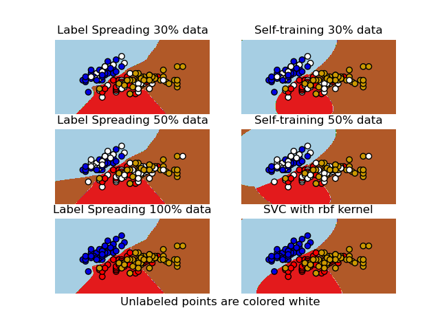
We observe that the decision boundaries are already quite similar to those using the full labeled data available for training, even when using a very small subset of the labels.
Interpretation of predict_proba#
predict_proba in LabelSpreading#
LabelSpreading constructs a similarity graph
from the data, by default using an RBF kernel. This means each sample is
connected to every other with a weight that decays with their squared
Euclidean distance, scaled by a parameter gamma.
Once we have that weighted graph, labels are propagated along the graph
edges. Each sample gradually takes on a soft label distribution that reflects
a weighted average of the labels of its neighbors until the process converges.
These per-sample distributions are stored in label_distributions_.
predict_proba computes the class probabilities for a new point by taking a
weighted average of the rows in label_distributions_, where the weights come
from the RBF kernel similarities between the new point and the training
samples. The averaged values are then renormalized so that they sum to one.
Just keep in mind that these “probabilities” are graph-based scores, not calibrated posteriors. Don’t over-interpret their absolute values.
from sklearn.metrics.pairwise import rbf_kernel

ls = ls100[0]  # fitted LabelSpreading instance
x_query = np.array([[3.5, 1.5]])  # point in the soft blue region

# Step 1: similarities between query and all training samples
W = rbf_kernel(x_query, X, gamma=ls.gamma)  # `gamma=20` by default

# Step 2: weighted average of label distributions
probs = np.dot(W, ls.label_distributions_)

# Step 3: normalize to sum to 1
probs /= probs.sum(axis=1, keepdims=True)

print("Manual:", probs)
print("API   :", ls.predict_proba(x_query))
Manual: [[0.96 0.03 0.01]]
API   : [[0.96 0.03 0.01]]
predict_proba in SelfTrainingClassifier#
SelfTrainingClassifier works by repeatedly
fitting its base estimator on the currently labeled data, then adding
pseudo-labels for unlabeled points whose predicted probabilities exceed a
confidence threshold. This process continues until no new points can be
labeled, at which point the classifier has a final fitted base estimator
stored in the attribute estimator_.
When you call predict_proba on the SelfTrainingClassifier, it simply
delegates to this final estimator.
st = st10[0]
print("Manual:", st.estimator_.predict_proba(x_query))
print("API   :", st.predict_proba(x_query))
Manual: [[0.41 0.37 0.22]]
API   : [[0.41 0.37 0.22]]
In both methods, semi-supervised learning can be understood as constructing a
categorical distribution over classes for each sample.
LabelSpreading keeps these distributions soft and
updates them through graph-based propagation.
Predictions (including predict_proba) remain tied to the training set, which
must be stored for inference.
SelfTrainingClassifier instead uses these
distributions internally to decide which unlabeled points to assign pseudo-labels
during training, but at prediction time the returned probabilities come directly from
the final fitted estimator, and therefore the decision rule does not require storing
the training data.
Total running time of the script: (0 minutes 1.685 seconds)
Related examples

Label Propagation digits: Demonstrating performance