Note
Go to the end to download the full example code or to run this example in your browser via JupyterLite or Binder.
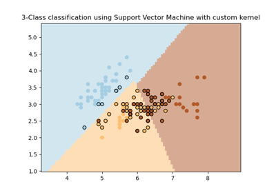
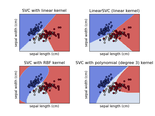
Plot different SVM classifiers in the iris dataset#
Comparison of different linear SVM classifiers on a 2D projection of the iris dataset. We only consider the first 2 features of this dataset:
Sepal length
Sepal width
This example shows how to plot the decision surface and the support vectors for four SVM classifiers with different kernels.
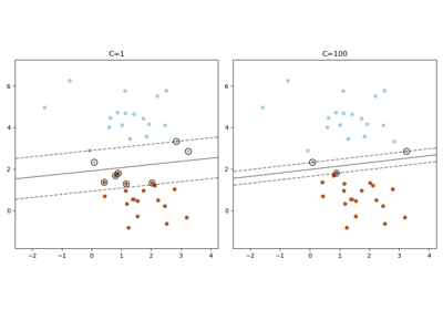
The linear models LinearSVC() and SVC(kernel='linear') yield slightly
different decision boundaries. This can be a consequence of the following
differences:
LinearSVCminimizes the squared hinge loss whileSVCminimizes the regular hinge loss.LinearSVCuses the One-vs-All (also known as One-vs-Rest) multiclass reduction whileSVCuses the One-vs-One multiclass reduction.
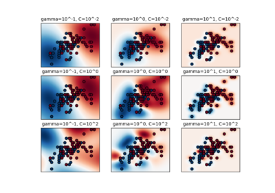
Both linear models have linear decision boundaries (intersecting hyperplanes) while the non-linear kernel models (polynomial or Gaussian RBF) have more flexible non-linear decision boundaries with shapes that depend on the kind of kernel and its parameters.
Note
While plotting the decision function of classifiers for toy 2D datasets can help get an intuitive understanding of their respective expressive power, be aware that those intuitions don’t always generalize to more realistic high-dimensional problems.
# Authors: The scikit-learn developers
# SPDX-License-Identifier: BSD-3-Clause

import matplotlib.pyplot as plt
import numpy as np

from sklearn import datasets, svm
from sklearn.inspection import DecisionBoundaryDisplay

# Import some data to play with.
iris = datasets.load_iris()
# Take the first two features. We could avoid this by using a two-dim dataset.
X = iris.data[:, :2]
y = iris.target

# We create an instance of SVM and fit out data. We do not scale our
# data since we want to plot the support vectors.
C = 1.0  # SVM regularization parameter
models = (
    svm.SVC(kernel="linear", C=C),
    svm.LinearSVC(C=C, max_iter=10000),
    svm.SVC(kernel="rbf", gamma=0.7, C=C),
    svm.SVC(kernel="poly", degree=3, gamma="auto", C=C),
)
models = (clf.fit(X, y) for clf in models)

# Title for the plots
titles = (
    "SVC with linear kernel",
    "LinearSVC (linear kernel)",
    "SVC with RBF kernel",
    "SVC with polynomial (degree 3) kernel",
)

# Set-up 2x2 grid for plotting.
fig, sub = plt.subplots(2, 2)
plt.subplots_adjust(wspace=0.4, hspace=0.4)

for clf, title, ax in zip(models, titles, sub.flatten()):
    disp = DecisionBoundaryDisplay.from_estimator(
        clf,
        X,
        response_method="predict",
        multiclass_colors="coolwarm",
        alpha=0.8,
        ax=ax,
        xlabel=iris.feature_names[0],
        ylabel=iris.feature_names[1],
    )

    # Plot the support vectors.
    # For LinearSVC we compute the support vectors from the decision function, see
    # https://scikit-learn.org/dev/auto_examples/svm/plot_linearsvc_support_vectors.html
    if hasattr(clf, "support_"):
        support_vector_indices = clf.support_
    else:
        decision_function = clf.decision_function(X)
        support_vector_indices = (np.abs(decision_function) <= 1 + 1e-15).nonzero()[0]
    ax.scatter(
        X[support_vector_indices, 0],
        X[support_vector_indices, 1],
        c=y[support_vector_indices],
        cmap=plt.cm.coolwarm,
        edgecolors="k",
    )

    ax.set_xticks(())
    ax.set_yticks(())
    ax.set_title(title)

plt.show()
Total running time of the script: (0 minutes 0.235 seconds)
Related examples