Note
Go to the end to download the full example code or to run this example in your browser via JupyterLite or Binder.
Adjustment for chance in clustering performance evaluation#
This notebook explores the impact of uniformly-distributed random labeling on the behavior of some clustering evaluation metrics. For such purpose, the metrics are computed with a fixed number of samples and as a function of the number of clusters assigned by the estimator. The example is divided into two experiments:
a first experiment with fixed “ground truth labels” (and therefore fixed number of classes) and randomly “predicted labels”;
a second experiment with varying “ground truth labels”, randomly “predicted labels”. The “predicted labels” have the same number of classes and clusters as the “ground truth labels”.
# Authors: The scikit-learn developers
# SPDX-License-Identifier: BSD-3-Clause
Defining the list of metrics to evaluate#
Clustering algorithms are fundamentally unsupervised learning methods. However, since we assign class labels for the synthetic clusters in this example, it is possible to use evaluation metrics that leverage this “supervised” ground truth information to quantify the quality of the resulting clusters. Examples of such metrics are the following:
V-measure, the harmonic mean of completeness and homogeneity;
Rand index, which measures how frequently pairs of data points are grouped consistently according to the result of the clustering algorithm and the ground truth class assignment;
Adjusted Rand index (ARI), a chance-adjusted Rand index such that a random cluster assignment has an ARI of 0.0 in expectation;
Mutual Information (MI) is an information theoretic measure that quantifies how dependent are the two labelings. Note that the maximum value of MI for perfect labelings depends on the number of clusters and samples;
Normalized Mutual Information (NMI), a Mutual Information defined between 0 (no mutual information) in the limit of large number of data points and 1 (perfectly matching label assignments, up to a permutation of the labels). It is not adjusted for chance: then the number of clustered data points is not large enough, the expected values of MI or NMI for random labelings can be significantly non-zero;
Adjusted Mutual Information (AMI), a chance-adjusted Mutual Information. Similarly to ARI, random cluster assignment has an AMI of 0.0 in expectation.
For more information, see the Clustering performance evaluation module.
from sklearn import metrics

score_funcs = [
    ("V-measure", metrics.v_measure_score),
    ("Rand index", metrics.rand_score),
    ("ARI", metrics.adjusted_rand_score),
    ("MI", metrics.mutual_info_score),
    ("NMI", metrics.normalized_mutual_info_score),
    ("AMI", metrics.adjusted_mutual_info_score),
]
First experiment: fixed ground truth labels and growing number of clusters#
We first define a function that creates uniformly-distributed random labeling.
import numpy as np

rng = np.random.RandomState(0)


def random_labels(n_samples, n_classes):
    return rng.randint(low=0, high=n_classes, size=n_samples)
Another function will use the random_labels function to create a fixed set
of ground truth labels (labels_a) distributed in n_classes and then score
several sets of randomly “predicted” labels (labels_b) to assess the
variability of a given metric at a given n_clusters.
def fixed_classes_uniform_labelings_scores(
    score_func, n_samples, n_clusters_range, n_classes, n_runs=5
):
    scores = np.zeros((len(n_clusters_range), n_runs))
    labels_a = random_labels(n_samples=n_samples, n_classes=n_classes)

    for i, n_clusters in enumerate(n_clusters_range):
        for j in range(n_runs):
            labels_b = random_labels(n_samples=n_samples, n_classes=n_clusters)
            scores[i, j] = score_func(labels_a, labels_b)
    return scores
In this first example we set the number of classes (true number of clusters) to
n_classes=10. The number of clusters varies over the values provided by
n_clusters_range.
import matplotlib.pyplot as plt
import seaborn as sns

n_samples = 1000
n_classes = 10
n_clusters_range = np.linspace(2, 100, 10).astype(int)
plots = []
names = []

sns.color_palette("colorblind")
plt.figure(1)

for marker, (score_name, score_func) in zip("d^vx.,", score_funcs):
    scores = fixed_classes_uniform_labelings_scores(
        score_func, n_samples, n_clusters_range, n_classes=n_classes
    )
    plots.append(
        plt.errorbar(
            n_clusters_range,
            scores.mean(axis=1),
            scores.std(axis=1),
            alpha=0.8,
            linewidth=1,
            marker=marker,
        )[0]
    )
    names.append(score_name)

plt.title(
    "Clustering measures for random uniform labeling\n"
    f"against reference assignment with {n_classes} classes"
)
plt.xlabel(f"Number of clusters (Number of samples is fixed to {n_samples})")
plt.ylabel("Score value")
plt.ylim(bottom=-0.05, top=1.05)
plt.legend(plots, names, bbox_to_anchor=(0.5, 0.5))
plt.show()
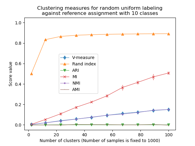
The Rand index saturates for n_clusters > n_classes. Other non-adjusted
measures such as the V-Measure show a linear dependency between the number of
clusters and the number of samples.
Adjusted for chance measure, such as ARI and AMI, display some random variations centered around a mean score of 0.0, independently of the number of samples and clusters.
Second experiment: varying number of classes and clusters#
In this section we define a similar function that uses several metrics to
score 2 uniformly-distributed random labelings. In this case, the number of
classes and assigned number of clusters are matched for each possible value in
n_clusters_range.
def uniform_labelings_scores(score_func, n_samples, n_clusters_range, n_runs=5):
    scores = np.zeros((len(n_clusters_range), n_runs))

    for i, n_clusters in enumerate(n_clusters_range):
        for j in range(n_runs):
            labels_a = random_labels(n_samples=n_samples, n_classes=n_clusters)
            labels_b = random_labels(n_samples=n_samples, n_classes=n_clusters)
            scores[i, j] = score_func(labels_a, labels_b)
    return scores
In this case, we use n_samples=100 to show the effect of having a number of
clusters similar or equal to the number of samples.
n_samples = 100
n_clusters_range = np.linspace(2, n_samples, 10).astype(int)

plt.figure(2)

plots = []
names = []

for marker, (score_name, score_func) in zip("d^vx.,", score_funcs):
    scores = uniform_labelings_scores(score_func, n_samples, n_clusters_range)
    plots.append(
        plt.errorbar(
            n_clusters_range,
            np.median(scores, axis=1),
            scores.std(axis=1),
            alpha=0.8,
            linewidth=2,
            marker=marker,
        )[0]
    )
    names.append(score_name)

plt.title(
    "Clustering measures for 2 random uniform labelings\nwith equal number of clusters"
)
plt.xlabel(f"Number of clusters (Number of samples is fixed to {n_samples})")
plt.ylabel("Score value")
plt.legend(plots, names)
plt.ylim(bottom=-0.05, top=1.05)
plt.show()
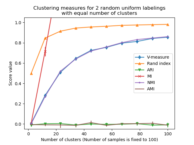
We observe similar results as for the first experiment: adjusted for chance metrics stay constantly near zero while other metrics tend to get larger with finer-grained labelings. The mean V-measure of random labeling increases significantly as the number of clusters is closer to the total number of samples used to compute the measure. Furthermore, raw Mutual Information is unbounded from above and its scale depends on the dimensions of the clustering problem and the cardinality of the ground truth classes. This is why the curve goes off the chart.
Only adjusted measures can hence be safely used as a consensus index to evaluate the average stability of clustering algorithms for a given value of k on various overlapping sub-samples of the dataset.
Non-adjusted clustering evaluation metric can therefore be misleading as they output large values for fine-grained labelings, one could be lead to think that the labeling has captured meaningful groups while they can be totally random. In particular, such non-adjusted metrics should not be used to compare the results of different clustering algorithms that output a different number of clusters.
Total running time of the script: (0 minutes 1.139 seconds)
Related examples
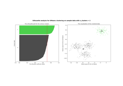
Selecting the number of clusters with silhouette analysis on KMeans clustering