Note
Go to the end to download the full example code or to run this example in your browser via JupyterLite or Binder.
Model-based and sequential feature selection#
This example illustrates and compares two approaches for feature selection:
SelectFromModel which is based on feature
importance, and
SequentialFeatureSelector which relies
on a greedy approach.
We use the Diabetes dataset, which consists of 10 features collected from 442 diabetes patients.
# Authors: The scikit-learn developers
# SPDX-License-Identifier: BSD-3-Clause
Loading the data#
We first load the diabetes dataset which is available from within scikit-learn, and print its description:
from sklearn.datasets import load_diabetes

diabetes = load_diabetes()
X, y = diabetes.data, diabetes.target
print(diabetes.DESCR)
.. _diabetes_dataset:

Diabetes dataset
----------------

Ten baseline variables, age, sex, body mass index, average blood
pressure, and six blood serum measurements were obtained for each of n =
442 diabetes patients, as well as the response of interest, a
quantitative measure of disease progression one year after baseline.

**Data Set Characteristics:**

:Number of Instances: 442

:Number of Attributes: First 10 columns are numeric predictive values

:Target: Column 11 is a quantitative measure of disease progression one year after baseline

:Attribute Information:
    - age     age in years
    - sex
    - bmi     body mass index
    - bp      average blood pressure
    - s1      tc, total serum cholesterol
    - s2      ldl, low-density lipoproteins
    - s3      hdl, high-density lipoproteins
    - s4      tch, total cholesterol / HDL
    - s5      ltg, possibly log of serum triglycerides level
    - s6      glu, blood sugar level

Note: Each of these 10 feature variables have been mean centered and scaled by the standard deviation times the square root of `n_samples` (i.e. the sum of squares of each column totals 1).

Source URL:
https://www4.stat.ncsu.edu/~boos/var.select/diabetes.html

For more information see:
Bradley Efron, Trevor Hastie, Iain Johnstone and Robert Tibshirani (2004) "Least Angle Regression," Annals of Statistics (with discussion), 407-499.
(https://web.stanford.edu/~hastie/Papers/LARS/LeastAngle_2002.pdf)
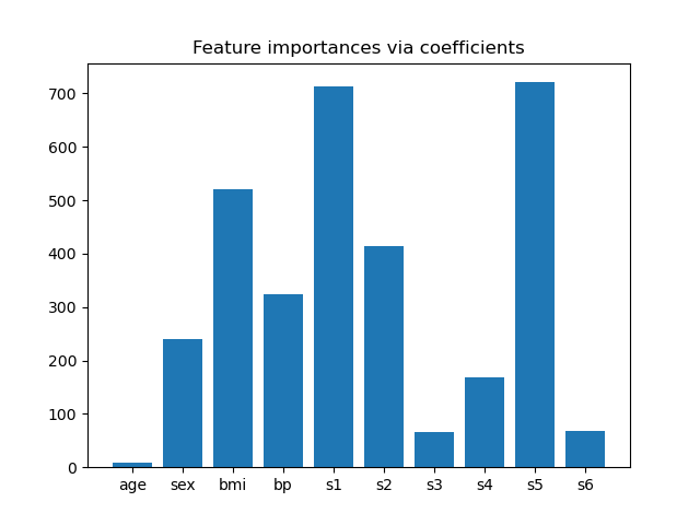
Feature importance from coefficients#
To get an idea of the importance of the features, we are going to use the
RidgeCV estimator. The features with the
highest absolute coef_ value are considered the most important.
We can observe the coefficients directly without needing to scale them (or
scale the data) because from the description above, we know that the features
were already standardized.
For a more complete example on the interpretations of the coefficients of
linear models, you may refer to
Common pitfalls in the interpretation of coefficients of linear models.
import matplotlib.pyplot as plt
import numpy as np

from sklearn.linear_model import RidgeCV

ridge = RidgeCV(alphas=np.logspace(-6, 6, num=5)).fit(X, y)
importance = np.abs(ridge.coef_)
feature_names = np.array(diabetes.feature_names)
plt.bar(height=importance, x=feature_names)
plt.title("Feature importances via coefficients")
plt.show()
Selecting features based on importance#
Now we want to select the two features which are the most important according
to the coefficients. The SelectFromModel
is meant just for that. SelectFromModel
accepts a threshold parameter and will select the features whose importance
(defined by the coefficients) are above this threshold.
Since we want to select only 2 features, we will set this threshold slightly above the coefficient of third most important feature.
from time import time

from sklearn.feature_selection import SelectFromModel

threshold = np.sort(importance)[-3] + 0.01

tic = time()
sfm = SelectFromModel(ridge, threshold=threshold).fit(X, y)
toc = time()
print(f"Features selected by SelectFromModel: {feature_names[sfm.get_support()]}")
print(f"Done in {toc - tic:.3f}s")
Features selected by SelectFromModel: ['s1' 's5']
Done in 0.002s
Selecting features with Sequential Feature Selection#
Another way of selecting features is to use
SequentialFeatureSelector
(SFS). SFS is a greedy procedure where, at each iteration, we choose the best
new feature to add to our selected features based a cross-validation score.
That is, we start with 0 features and choose the best single feature with the
highest score. The procedure is repeated until we reach the desired number of
selected features.
We can also go in the reverse direction (backward SFS), i.e. start with all the features and greedily choose features to remove one by one. We illustrate both approaches here.
from sklearn.feature_selection import SequentialFeatureSelector

tic_fwd = time()
sfs_forward = SequentialFeatureSelector(
    ridge, n_features_to_select=2, direction="forward"
).fit(X, y)
toc_fwd = time()

tic_bwd = time()
sfs_backward = SequentialFeatureSelector(
    ridge, n_features_to_select=2, direction="backward"
).fit(X, y)
toc_bwd = time()

print(
    "Features selected by forward sequential selection: "
    f"{feature_names[sfs_forward.get_support()]}"
)
print(f"Done in {toc_fwd - tic_fwd:.3f}s")
print(
    "Features selected by backward sequential selection: "
    f"{feature_names[sfs_backward.get_support()]}"
)
print(f"Done in {toc_bwd - tic_bwd:.3f}s")
Features selected by forward sequential selection: ['bmi' 's5']
Done in 0.202s
Features selected by backward sequential selection: ['bmi' 's5']
Done in 0.607s
Interestingly, forward and backward selection have selected the same set of features. In general, this isn’t the case and the two methods would lead to different results.
We also note that the features selected by SFS differ from those selected by
feature importance: SFS selects bmi instead of s1. This does sound
reasonable though, since bmi corresponds to the third most important
feature according to the coefficients. It is quite remarkable considering
that SFS makes no use of the coefficients at all.
To finish with, we should note that
SelectFromModel is significantly faster
than SFS. Indeed, SelectFromModel only
needs to fit a model once, while SFS needs to cross-validate many different
models for each of the iterations. SFS however works with any model, while
SelectFromModel requires the underlying
estimator to expose a coef_ attribute or a feature_importances_
attribute. The forward SFS is faster than the backward SFS because it only
needs to perform n_features_to_select = 2 iterations, while the backward
SFS needs to perform n_features - n_features_to_select = 8 iterations.
Using negative tolerance values#
SequentialFeatureSelector can be used
to remove features present in the dataset and return a
smaller subset of the original features with direction="backward"
and a negative value of tol.
We begin by loading the Breast Cancer dataset, consisting of 30 different features and 569 samples.
import numpy as np

from sklearn.datasets import load_breast_cancer

breast_cancer_data = load_breast_cancer()
X, y = breast_cancer_data.data, breast_cancer_data.target
feature_names = np.array(breast_cancer_data.feature_names)
print(breast_cancer_data.DESCR)
.. _breast_cancer_dataset:

Breast cancer Wisconsin (diagnostic) dataset
--------------------------------------------

**Data Set Characteristics:**

:Number of Instances: 569

:Number of Attributes: 30 numeric, predictive attributes and the class

:Attribute Information:
    - radius (mean of distances from center to points on the perimeter)
    - texture (standard deviation of gray-scale values)
    - perimeter
    - area
    - smoothness (local variation in radius lengths)
    - compactness (perimeter^2 / area - 1.0)
    - concavity (severity of concave portions of the contour)
    - concave points (number of concave portions of the contour)
    - symmetry
    - fractal dimension ("coastline approximation" - 1)

    The mean, standard error, and "worst" or largest (mean of the three
    worst/largest values) of these features were computed for each image,
    resulting in 30 features.  For instance, field 0 is Mean Radius, field
    10 is Radius SE, field 20 is Worst Radius.

    - class:
            - WDBC-Malignant
            - WDBC-Benign

:Summary Statistics:

===================================== ====== ======
                                        Min    Max
===================================== ====== ======
radius (mean):                        6.981  28.11
texture (mean):                       9.71   39.28
perimeter (mean):                     43.79  188.5
area (mean):                          143.5  2501.0
smoothness (mean):                    0.053  0.163
compactness (mean):                   0.019  0.345
concavity (mean):                     0.0    0.427
concave points (mean):                0.0    0.201
symmetry (mean):                      0.106  0.304
fractal dimension (mean):             0.05   0.097
radius (standard error):              0.112  2.873
texture (standard error):             0.36   4.885
perimeter (standard error):           0.757  21.98
area (standard error):                6.802  542.2
smoothness (standard error):          0.002  0.031
compactness (standard error):         0.002  0.135
concavity (standard error):           0.0    0.396
concave points (standard error):      0.0    0.053
symmetry (standard error):            0.008  0.079
fractal dimension (standard error):   0.001  0.03
radius (worst):                       7.93   36.04
texture (worst):                      12.02  49.54
perimeter (worst):                    50.41  251.2
area (worst):                         185.2  4254.0
smoothness (worst):                   0.071  0.223
compactness (worst):                  0.027  1.058
concavity (worst):                    0.0    1.252
concave points (worst):               0.0    0.291
symmetry (worst):                     0.156  0.664
fractal dimension (worst):            0.055  0.208
===================================== ====== ======

:Missing Attribute Values: None

:Class Distribution: 212 - Malignant, 357 - Benign

:Creator:  Dr. William H. Wolberg, W. Nick Street, Olvi L. Mangasarian

:Donor: Nick Street

:Date: November, 1995

This is a copy of UCI ML Breast Cancer Wisconsin (Diagnostic) datasets.
https://goo.gl/U2Uwz2

Features are computed from a digitized image of a fine needle
aspirate (FNA) of a breast mass.  They describe
characteristics of the cell nuclei present in the image.

Separating plane described above was obtained using
Multisurface Method-Tree (MSM-T) [K. P. Bennett, "Decision Tree
Construction Via Linear Programming." Proceedings of the 4th
Midwest Artificial Intelligence and Cognitive Science Society,
pp. 97-101, 1992], a classification method which uses linear
programming to construct a decision tree.  Relevant features
were selected using an exhaustive search in the space of 1-4
features and 1-3 separating planes.

The actual linear program used to obtain the separating plane
in the 3-dimensional space is that described in:
[K. P. Bennett and O. L. Mangasarian: "Robust Linear
Programming Discrimination of Two Linearly Inseparable Sets",
Optimization Methods and Software 1, 1992, 23-34].

This database is also available through the UW CS ftp server:

ftp ftp.cs.wisc.edu
cd math-prog/cpo-dataset/machine-learn/WDBC/

.. dropdown:: References

  - W.N. Street, W.H. Wolberg and O.L. Mangasarian. Nuclear feature extraction
    for breast tumor diagnosis. IS&T/SPIE 1993 International Symposium on
    Electronic Imaging: Science and Technology, volume 1905, pages 861-870,
    San Jose, CA, 1993.
  - O.L. Mangasarian, W.N. Street and W.H. Wolberg. Breast cancer diagnosis and
    prognosis via linear programming. Operations Research, 43(4), pages 570-577,
    July-August 1995.
  - W.H. Wolberg, W.N. Street, and O.L. Mangasarian. Machine learning techniques
    to diagnose breast cancer from fine-needle aspirates. Cancer Letters 77 (1994)
    163-171.
We will make use of the LogisticRegression
estimator with SequentialFeatureSelector
to perform the feature selection.
from sklearn.linear_model import LogisticRegression
from sklearn.metrics import roc_auc_score
from sklearn.pipeline import make_pipeline
from sklearn.preprocessing import StandardScaler

for tol in [-1e-2, -1e-3, -1e-4]:
    start = time()
    feature_selector = SequentialFeatureSelector(
        LogisticRegression(),
        n_features_to_select="auto",
        direction="backward",
        scoring="roc_auc",
        tol=tol,
        n_jobs=2,
    )
    model = make_pipeline(StandardScaler(), feature_selector, LogisticRegression())
    model.fit(X, y)
    end = time()
    print(f"\ntol: {tol}")
    print(f"Features selected: {feature_names[model[1].get_support()]}")
    print(f"ROC AUC score: {roc_auc_score(y, model.predict_proba(X)[:, 1]):.3f}")
    print(f"Done in {end - start:.3f}s")
tol: -0.01
Features selected: ['worst perimeter']
ROC AUC score: 0.975
Done in 16.976s

tol: -0.001
Features selected: ['radius error' 'fractal dimension error' 'worst texture'
 'worst perimeter' 'worst concave points']
ROC AUC score: 0.997
Done in 17.887s

tol: -0.0001
Features selected: ['mean compactness' 'mean concavity' 'mean concave points' 'radius error'
 'area error' 'concave points error' 'symmetry error'
 'fractal dimension error' 'worst texture' 'worst perimeter' 'worst area'
 'worst concave points' 'worst symmetry']
ROC AUC score: 0.998
Done in 17.024s
We can see that the number of features selected tend to increase as negative
values of tol approach to zero. The time taken for feature selection also
decreases as the values of tol come closer to zero.
Total running time of the script: (0 minutes 52.793 seconds)
Related examples

Post-hoc tuning the cut-off point of decision function
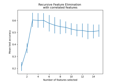
Recursive feature elimination with cross-validation
