Note
Go to the end to download the full example code or to run this example in your browser via JupyterLite or Binder.
Faces dataset decompositions#
This example applies to The Olivetti faces dataset different unsupervised
matrix decomposition (dimension reduction) methods from the module
sklearn.decomposition (see the documentation chapter
Decomposing signals in components (matrix factorization problems)).
# Authors: The scikit-learn developers
# SPDX-License-Identifier: BSD-3-Clause
Dataset preparation#
Loading and preprocessing the Olivetti faces dataset.
import logging

import matplotlib.pyplot as plt
from numpy.random import RandomState

from sklearn import cluster, decomposition
from sklearn.datasets import fetch_olivetti_faces

rng = RandomState(0)

# Display progress logs on stdout
logging.basicConfig(level=logging.INFO, format="%(asctime)s %(levelname)s %(message)s")

faces, _ = fetch_olivetti_faces(return_X_y=True, shuffle=True, random_state=rng)
n_samples, n_features = faces.shape

# Global centering (focus on one feature, centering all samples)
faces_centered = faces - faces.mean(axis=0)

# Local centering (focus on one sample, centering all features)
faces_centered -= faces_centered.mean(axis=1).reshape(n_samples, -1)

print("Dataset consists of %d faces" % n_samples)
Dataset consists of 400 faces
Define a base function to plot the gallery of faces.
n_row, n_col = 2, 3
n_components = n_row * n_col
image_shape = (64, 64)


def plot_gallery(title, images, n_col=n_col, n_row=n_row, cmap=plt.cm.gray):
    fig, axs = plt.subplots(
        nrows=n_row,
        ncols=n_col,
        figsize=(2.0 * n_col, 2.3 * n_row),
        facecolor="white",
        constrained_layout=True,
    )
    fig.get_layout_engine().set(w_pad=0.01, h_pad=0.02, hspace=0, wspace=0)
    fig.set_edgecolor("black")
    fig.suptitle(title, size=16)
    for ax, vec in zip(axs.flat, images):
        vmax = max(vec.max(), -vec.min())
        im = ax.imshow(
            vec.reshape(image_shape),
            cmap=cmap,
            interpolation="nearest",
            vmin=-vmax,
            vmax=vmax,
        )
        ax.axis("off")

    fig.colorbar(im, ax=axs, orientation="horizontal", shrink=0.99, aspect=40, pad=0.01)
    plt.show()
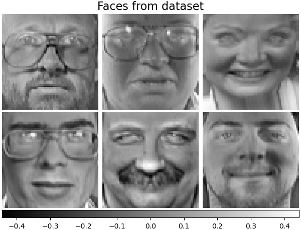
Let’s take a look at our data. Gray color indicates negative values, white indicates positive values.
plot_gallery("Faces from dataset", faces_centered[:n_components])
Decomposition#
Initialise different estimators for decomposition and fit each of them on all images and plot some results. Each estimator extracts 6 components as vectors \(h \in \mathbb{R}^{4096}\). We just displayed these vectors in human-friendly visualisation as 64x64 pixel images.
Read more in the User Guide.
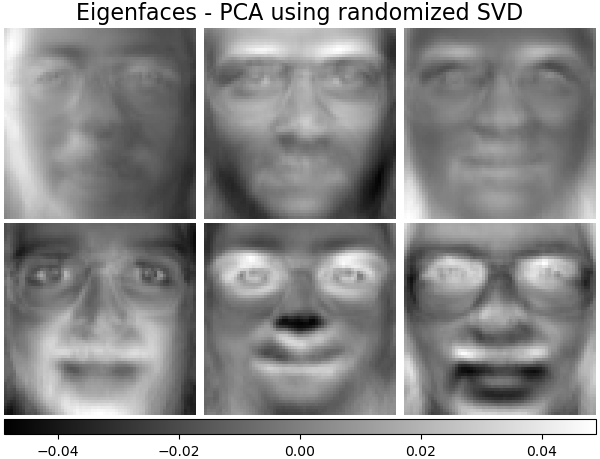
Eigenfaces - PCA using randomized SVD#
Linear dimensionality reduction using Singular Value Decomposition (SVD) of the data to project it to a lower dimensional space.
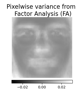
Note
The Eigenfaces estimator, via the sklearn.decomposition.PCA,
also provides a scalar noise_variance_ (the mean of pixelwise variance)
that cannot be displayed as an image.
pca_estimator = decomposition.PCA(
    n_components=n_components, svd_solver="randomized", whiten=True
)
pca_estimator.fit(faces_centered)
plot_gallery(
    "Eigenfaces - PCA using randomized SVD", pca_estimator.components_[:n_components]
)
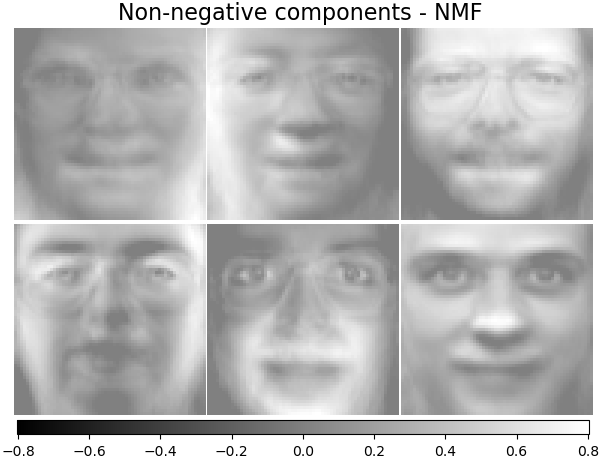
Non-negative components - NMF#
Estimate non-negative original data as production of two non-negative matrices.
nmf_estimator = decomposition.NMF(n_components=n_components, tol=5e-3)
nmf_estimator.fit(faces)  # original non- negative dataset
plot_gallery("Non-negative components - NMF", nmf_estimator.components_[:n_components])
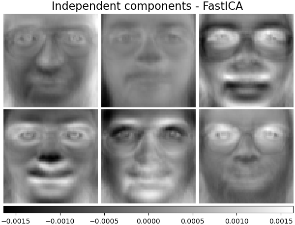
Independent components - FastICA#
Independent component analysis separates a multivariate vectors into additive subcomponents that are maximally independent.
ica_estimator = decomposition.FastICA(
    n_components=n_components, max_iter=400, whiten="arbitrary-variance", tol=15e-5
)
ica_estimator.fit(faces_centered)
plot_gallery(
    "Independent components - FastICA", ica_estimator.components_[:n_components]
)
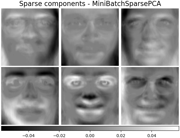
Sparse components - MiniBatchSparsePCA#
Mini-batch sparse PCA (MiniBatchSparsePCA)
extracts the set of sparse components that best reconstruct the data. This
variant is faster but less accurate than the similar
SparsePCA.
batch_pca_estimator = decomposition.MiniBatchSparsePCA(
    n_components=n_components, alpha=0.1, max_iter=100, batch_size=3, random_state=rng
)
batch_pca_estimator.fit(faces_centered)
plot_gallery(
    "Sparse components - MiniBatchSparsePCA",
    batch_pca_estimator.components_[:n_components],
)
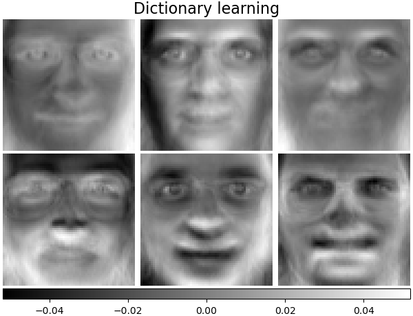
Dictionary learning#
By default, MiniBatchDictionaryLearning
divides the data into mini-batches and optimizes in an online manner by
cycling over the mini-batches for the specified number of iterations.
batch_dict_estimator = decomposition.MiniBatchDictionaryLearning(
    n_components=n_components, alpha=0.1, max_iter=50, batch_size=3, random_state=rng
)
batch_dict_estimator.fit(faces_centered)
plot_gallery("Dictionary learning", batch_dict_estimator.components_[:n_components])
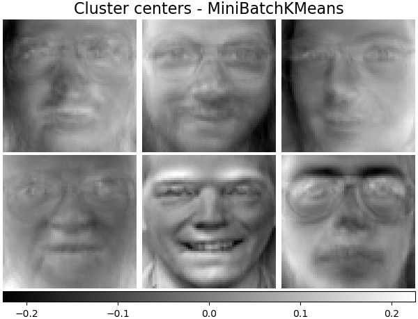
Cluster centers - MiniBatchKMeans#
sklearn.cluster.MiniBatchKMeans is computationally efficient and
implements on-line learning with a
partial_fit method. That is
why it could be beneficial to enhance some time-consuming algorithms with
MiniBatchKMeans.
kmeans_estimator = cluster.MiniBatchKMeans(
    n_clusters=n_components,
    tol=1e-3,
    batch_size=20,
    max_iter=50,
    random_state=rng,
)
kmeans_estimator.fit(faces_centered)
plot_gallery(
    "Cluster centers - MiniBatchKMeans",
    kmeans_estimator.cluster_centers_[:n_components],
)
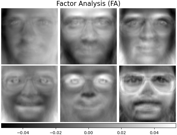
Factor Analysis components - FA#
FactorAnalysis is similar to
PCA but has the advantage of modelling the
variance in every direction of the input space independently (heteroscedastic
noise). Read more in the User Guide.
fa_estimator = decomposition.FactorAnalysis(n_components=n_components, max_iter=20)
fa_estimator.fit(faces_centered)
plot_gallery("Factor Analysis (FA)", fa_estimator.components_[:n_components])

# --- Pixelwise variance
plt.figure(figsize=(3.2, 3.6), facecolor="white", tight_layout=True)
vec = fa_estimator.noise_variance_
vmax = max(vec.max(), -vec.min())
plt.imshow(
    vec.reshape(image_shape),
    cmap=plt.cm.gray,
    interpolation="nearest",
    vmin=-vmax,
    vmax=vmax,
)
plt.axis("off")
plt.title("Pixelwise variance from \n Factor Analysis (FA)", size=16, wrap=True)
plt.colorbar(orientation="horizontal", shrink=0.8, pad=0.03)
plt.show()
Decomposition: Dictionary learning#
In the further section, let’s consider Dictionary Learning more precisely. Dictionary learning is a problem that amounts to finding a sparse representation of the input data as a combination of simple elements. These simple elements form a dictionary. It is possible to constrain the dictionary and/or coding coefficients to be positive to match constraints that may be present in the data.
MiniBatchDictionaryLearning implements a
faster, but less accurate version of the dictionary learning algorithm that
is better suited for large datasets. Read more in the User Guide.
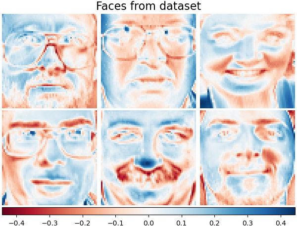
Plot the same samples from our dataset but with another colormap. Red indicates negative values, blue indicates positive values, and white represents zeros.
plot_gallery("Faces from dataset", faces_centered[:n_components], cmap=plt.cm.RdBu)
Similar to the previous examples, we change parameters and train
MiniBatchDictionaryLearning estimator on all
images. Generally, the dictionary learning and sparse encoding decompose
input data into the dictionary and the coding coefficients matrices. \(X
\approx UV\), where \(X = [x_1, . . . , x_n]\), \(X \in
\mathbb{R}^{m×n}\), dictionary \(U \in \mathbb{R}^{m×k}\), coding
coefficients \(V \in \mathbb{R}^{k×n}\).
Also below are the results when the dictionary and coding coefficients are positively constrained.
Dictionary learning - positive dictionary#
In the following section we enforce positivity when finding the dictionary.
dict_pos_dict_estimator = decomposition.MiniBatchDictionaryLearning(
    n_components=n_components,
    alpha=0.1,
    max_iter=50,
    batch_size=3,
    random_state=rng,
    positive_dict=True,
)
dict_pos_dict_estimator.fit(faces_centered)
plot_gallery(
    "Dictionary learning - positive dictionary",
    dict_pos_dict_estimator.components_[:n_components],
    cmap=plt.cm.RdBu,
)

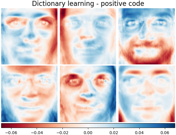
Dictionary learning - positive code#
Below we constrain the coding coefficients as a positive matrix.
dict_pos_code_estimator = decomposition.MiniBatchDictionaryLearning(
    n_components=n_components,
    alpha=0.1,
    max_iter=50,
    batch_size=3,
    fit_algorithm="cd",
    random_state=rng,
    positive_code=True,
)
dict_pos_code_estimator.fit(faces_centered)
plot_gallery(
    "Dictionary learning - positive code",
    dict_pos_code_estimator.components_[:n_components],
    cmap=plt.cm.RdBu,
)
/home/circleci/project/sklearn/linear_model/_coordinate_descent.py:825: ConvergenceWarning: Objective did not converge. You might want to increase the number of iterations, check the scale of the features or consider increasing regularisation. Duality gap: 1.907349e-06, tolerance: 3.737e-07
  model = cd_fast.enet_coordinate_descent_gram(
/home/circleci/project/sklearn/linear_model/_coordinate_descent.py:825: ConvergenceWarning: Objective did not converge. You might want to increase the number of iterations, check the scale of the features or consider increasing regularisation. Duality gap: 3.814697e-06, tolerance: 8.344e-07
  model = cd_fast.enet_coordinate_descent_gram(
/home/circleci/project/sklearn/linear_model/_coordinate_descent.py:825: ConvergenceWarning: Objective did not converge. You might want to increase the number of iterations, check the scale of the features or consider increasing regularisation. Duality gap: 3.814697e-06, tolerance: 4.820e-07
  model = cd_fast.enet_coordinate_descent_gram(
/home/circleci/project/sklearn/linear_model/_coordinate_descent.py:825: ConvergenceWarning: Objective did not converge. You might want to increase the number of iterations, check the scale of the features or consider increasing regularisation. Duality gap: 1.907349e-06, tolerance: 3.218e-07
  model = cd_fast.enet_coordinate_descent_gram(
/home/circleci/project/sklearn/linear_model/_coordinate_descent.py:825: ConvergenceWarning: Objective did not converge. You might want to increase the number of iterations, check the scale of the features or consider increasing regularisation. Duality gap: 1.907349e-06, tolerance: 3.449e-07
  model = cd_fast.enet_coordinate_descent_gram(
/home/circleci/project/sklearn/linear_model/_coordinate_descent.py:825: ConvergenceWarning: Objective did not converge. You might want to increase the number of iterations, check the scale of the features or consider increasing regularisation. Duality gap: 3.814697e-06, tolerance: 6.049e-07
  model = cd_fast.enet_coordinate_descent_gram(
/home/circleci/project/sklearn/linear_model/_coordinate_descent.py:825: ConvergenceWarning: Objective did not converge. You might want to increase the number of iterations, check the scale of the features or consider increasing regularisation. Duality gap: 1.144409e-05, tolerance: 8.649e-07
  model = cd_fast.enet_coordinate_descent_gram(
/home/circleci/project/sklearn/linear_model/_coordinate_descent.py:825: ConvergenceWarning: Objective did not converge. You might want to increase the number of iterations, check the scale of the features or consider increasing regularisation. Duality gap: 3.814697e-06, tolerance: 5.296e-07
  model = cd_fast.enet_coordinate_descent_gram(
/home/circleci/project/sklearn/linear_model/_coordinate_descent.py:825: ConvergenceWarning: Objective did not converge. You might want to increase the number of iterations, check the scale of the features or consider increasing regularisation. Duality gap: 3.814697e-06, tolerance: 7.128e-07
  model = cd_fast.enet_coordinate_descent_gram(
/home/circleci/project/sklearn/linear_model/_coordinate_descent.py:825: ConvergenceWarning: Objective did not converge. You might want to increase the number of iterations, check the scale of the features or consider increasing regularisation. Duality gap: 1.907349e-06, tolerance: 6.210e-07
  model = cd_fast.enet_coordinate_descent_gram(
/home/circleci/project/sklearn/linear_model/_coordinate_descent.py:825: ConvergenceWarning: Objective did not converge. You might want to increase the number of iterations, check the scale of the features or consider increasing regularisation. Duality gap: 7.629395e-06, tolerance: 1.127e-06
  model = cd_fast.enet_coordinate_descent_gram(
/home/circleci/project/sklearn/linear_model/_coordinate_descent.py:825: ConvergenceWarning: Objective did not converge. You might want to increase the number of iterations, check the scale of the features or consider increasing regularisation. Duality gap: 3.814697e-06, tolerance: 6.651e-07
  model = cd_fast.enet_coordinate_descent_gram(
/home/circleci/project/sklearn/linear_model/_coordinate_descent.py:825: ConvergenceWarning: Objective did not converge. You might want to increase the number of iterations, check the scale of the features or consider increasing regularisation. Duality gap: 1.907349e-06, tolerance: 5.710e-07
  model = cd_fast.enet_coordinate_descent_gram(
/home/circleci/project/sklearn/linear_model/_coordinate_descent.py:825: ConvergenceWarning: Objective did not converge. You might want to increase the number of iterations, check the scale of the features or consider increasing regularisation. Duality gap: 2.861023e-06, tolerance: 6.737e-07
  model = cd_fast.enet_coordinate_descent_gram(
/home/circleci/project/sklearn/linear_model/_coordinate_descent.py:825: ConvergenceWarning: Objective did not converge. You might want to increase the number of iterations, check the scale of the features or consider increasing regularisation. Duality gap: 7.629395e-06, tolerance: 8.669e-07
  model = cd_fast.enet_coordinate_descent_gram(
/home/circleci/project/sklearn/linear_model/_coordinate_descent.py:825: ConvergenceWarning: Objective did not converge. You might want to increase the number of iterations, check the scale of the features or consider increasing regularisation. Duality gap: 5.722046e-06, tolerance: 8.331e-07
  model = cd_fast.enet_coordinate_descent_gram(
/home/circleci/project/sklearn/linear_model/_coordinate_descent.py:825: ConvergenceWarning: Objective did not converge. You might want to increase the number of iterations, check the scale of the features or consider increasing regularisation. Duality gap: 3.814697e-06, tolerance: 3.817e-07
  model = cd_fast.enet_coordinate_descent_gram(
/home/circleci/project/sklearn/linear_model/_coordinate_descent.py:825: ConvergenceWarning: Objective did not converge. You might want to increase the number of iterations, check the scale of the features or consider increasing regularisation. Duality gap: 9.536743e-06, tolerance: 1.173e-06
  model = cd_fast.enet_coordinate_descent_gram(
/home/circleci/project/sklearn/linear_model/_coordinate_descent.py:825: ConvergenceWarning: Objective did not converge. You might want to increase the number of iterations, check the scale of the features or consider increasing regularisation. Duality gap: 9.536743e-07, tolerance: 2.379e-07
  model = cd_fast.enet_coordinate_descent_gram(
/home/circleci/project/sklearn/linear_model/_coordinate_descent.py:825: ConvergenceWarning: Objective did not converge. You might want to increase the number of iterations, check the scale of the features or consider increasing regularisation. Duality gap: 3.814697e-06, tolerance: 6.859e-07
  model = cd_fast.enet_coordinate_descent_gram(
/home/circleci/project/sklearn/linear_model/_coordinate_descent.py:825: ConvergenceWarning: Objective did not converge. You might want to increase the number of iterations, check the scale of the features or consider increasing regularisation. Duality gap: 1.907349e-06, tolerance: 2.167e-07
  model = cd_fast.enet_coordinate_descent_gram(
/home/circleci/project/sklearn/linear_model/_coordinate_descent.py:825: ConvergenceWarning: Objective did not converge. You might want to increase the number of iterations, check the scale of the features or consider increasing regularisation. Duality gap: 1.907349e-06, tolerance: 3.649e-07
  model = cd_fast.enet_coordinate_descent_gram(
/home/circleci/project/sklearn/linear_model/_coordinate_descent.py:825: ConvergenceWarning: Objective did not converge. You might want to increase the number of iterations, check the scale of the features or consider increasing regularisation. Duality gap: 3.814697e-06, tolerance: 9.119e-07
  model = cd_fast.enet_coordinate_descent_gram(
/home/circleci/project/sklearn/linear_model/_coordinate_descent.py:825: ConvergenceWarning: Objective did not converge. You might want to increase the number of iterations, check the scale of the features or consider increasing regularisation. Duality gap: 3.814697e-06, tolerance: 5.653e-07
  model = cd_fast.enet_coordinate_descent_gram(
/home/circleci/project/sklearn/linear_model/_coordinate_descent.py:825: ConvergenceWarning: Objective did not converge. You might want to increase the number of iterations, check the scale of the features or consider increasing regularisation. Duality gap: 9.536743e-07, tolerance: 6.697e-07
  model = cd_fast.enet_coordinate_descent_gram(
/home/circleci/project/sklearn/linear_model/_coordinate_descent.py:825: ConvergenceWarning: Objective did not converge. You might want to increase the number of iterations, check the scale of the features or consider increasing regularisation. Duality gap: 3.814697e-06, tolerance: 3.944e-07
  model = cd_fast.enet_coordinate_descent_gram(
/home/circleci/project/sklearn/linear_model/_coordinate_descent.py:825: ConvergenceWarning: Objective did not converge. You might want to increase the number of iterations, check the scale of the features or consider increasing regularisation. Duality gap: 3.814697e-06, tolerance: 7.156e-07
  model = cd_fast.enet_coordinate_descent_gram(
/home/circleci/project/sklearn/linear_model/_coordinate_descent.py:825: ConvergenceWarning: Objective did not converge. You might want to increase the number of iterations, check the scale of the features or consider increasing regularisation. Duality gap: 9.536743e-07, tolerance: 2.532e-07
  model = cd_fast.enet_coordinate_descent_gram(
/home/circleci/project/sklearn/linear_model/_coordinate_descent.py:825: ConvergenceWarning: Objective did not converge. You might want to increase the number of iterations, check the scale of the features or consider increasing regularisation. Duality gap: 3.814697e-06, tolerance: 1.198e-06
  model = cd_fast.enet_coordinate_descent_gram(
/home/circleci/project/sklearn/linear_model/_coordinate_descent.py:825: ConvergenceWarning: Objective did not converge. You might want to increase the number of iterations, check the scale of the features or consider increasing regularisation. Duality gap: 1.525879e-05, tolerance: 1.527e-06
  model = cd_fast.enet_coordinate_descent_gram(
/home/circleci/project/sklearn/linear_model/_coordinate_descent.py:825: ConvergenceWarning: Objective did not converge. You might want to increase the number of iterations, check the scale of the features or consider increasing regularisation. Duality gap: 3.814697e-06, tolerance: 1.163e-06
  model = cd_fast.enet_coordinate_descent_gram(
/home/circleci/project/sklearn/linear_model/_coordinate_descent.py:825: ConvergenceWarning: Objective did not converge. You might want to increase the number of iterations, check the scale of the features or consider increasing regularisation. Duality gap: 3.814697e-06, tolerance: 4.891e-07
  model = cd_fast.enet_coordinate_descent_gram(
/home/circleci/project/sklearn/linear_model/_coordinate_descent.py:825: ConvergenceWarning: Objective did not converge. You might want to increase the number of iterations, check the scale of the features or consider increasing regularisation. Duality gap: 3.814697e-06, tolerance: 4.796e-07
  model = cd_fast.enet_coordinate_descent_gram(
/home/circleci/project/sklearn/linear_model/_coordinate_descent.py:825: ConvergenceWarning: Objective did not converge. You might want to increase the number of iterations, check the scale of the features or consider increasing regularisation. Duality gap: 3.814697e-06, tolerance: 7.107e-07
  model = cd_fast.enet_coordinate_descent_gram(
/home/circleci/project/sklearn/linear_model/_coordinate_descent.py:825: ConvergenceWarning: Objective did not converge. You might want to increase the number of iterations, check the scale of the features or consider increasing regularisation. Duality gap: 2.861023e-06, tolerance: 4.261e-07
  model = cd_fast.enet_coordinate_descent_gram(
/home/circleci/project/sklearn/linear_model/_coordinate_descent.py:825: ConvergenceWarning: Objective did not converge. You might want to increase the number of iterations, check the scale of the features or consider increasing regularisation. Duality gap: 1.907349e-06, tolerance: 8.734e-07
  model = cd_fast.enet_coordinate_descent_gram(
/home/circleci/project/sklearn/linear_model/_coordinate_descent.py:825: ConvergenceWarning: Objective did not converge. You might want to increase the number of iterations, check the scale of the features or consider increasing regularisation. Duality gap: 3.814697e-06, tolerance: 6.358e-07
  model = cd_fast.enet_coordinate_descent_gram(
/home/circleci/project/sklearn/linear_model/_coordinate_descent.py:825: ConvergenceWarning: Objective did not converge. You might want to increase the number of iterations, check the scale of the features or consider increasing regularisation. Duality gap: 1.907349e-06, tolerance: 6.932e-07
  model = cd_fast.enet_coordinate_descent_gram(
/home/circleci/project/sklearn/linear_model/_coordinate_descent.py:825: ConvergenceWarning: Objective did not converge. You might want to increase the number of iterations, check the scale of the features or consider increasing regularisation. Duality gap: 3.814697e-06, tolerance: 8.329e-07
  model = cd_fast.enet_coordinate_descent_gram(
/home/circleci/project/sklearn/linear_model/_coordinate_descent.py:825: ConvergenceWarning: Objective did not converge. You might want to increase the number of iterations, check the scale of the features or consider increasing regularisation. Duality gap: 5.722046e-06, tolerance: 7.010e-07
  model = cd_fast.enet_coordinate_descent_gram(
/home/circleci/project/sklearn/linear_model/_coordinate_descent.py:825: ConvergenceWarning: Objective did not converge. You might want to increase the number of iterations, check the scale of the features or consider increasing regularisation. Duality gap: 7.629395e-06, tolerance: 6.543e-07
  model = cd_fast.enet_coordinate_descent_gram(
/home/circleci/project/sklearn/linear_model/_coordinate_descent.py:825: ConvergenceWarning: Objective did not converge. You might want to increase the number of iterations, check the scale of the features or consider increasing regularisation. Duality gap: 3.814697e-06, tolerance: 5.837e-07
  model = cd_fast.enet_coordinate_descent_gram(
/home/circleci/project/sklearn/linear_model/_coordinate_descent.py:825: ConvergenceWarning: Objective did not converge. You might want to increase the number of iterations, check the scale of the features or consider increasing regularisation. Duality gap: 1.335144e-05, tolerance: 8.823e-07
  model = cd_fast.enet_coordinate_descent_gram(
/home/circleci/project/sklearn/linear_model/_coordinate_descent.py:825: ConvergenceWarning: Objective did not converge. You might want to increase the number of iterations, check the scale of the features or consider increasing regularisation. Duality gap: 3.814697e-06, tolerance: 6.943e-07
  model = cd_fast.enet_coordinate_descent_gram(
/home/circleci/project/sklearn/linear_model/_coordinate_descent.py:825: ConvergenceWarning: Objective did not converge. You might want to increase the number of iterations, check the scale of the features or consider increasing regularisation. Duality gap: 1.907349e-06, tolerance: 9.927e-07
  model = cd_fast.enet_coordinate_descent_gram(
/home/circleci/project/sklearn/linear_model/_coordinate_descent.py:825: ConvergenceWarning: Objective did not converge. You might want to increase the number of iterations, check the scale of the features or consider increasing regularisation. Duality gap: 9.536743e-07, tolerance: 3.557e-07
  model = cd_fast.enet_coordinate_descent_gram(
/home/circleci/project/sklearn/linear_model/_coordinate_descent.py:825: ConvergenceWarning: Objective did not converge. You might want to increase the number of iterations, check the scale of the features or consider increasing regularisation. Duality gap: 3.814697e-06, tolerance: 7.508e-07
  model = cd_fast.enet_coordinate_descent_gram(
/home/circleci/project/sklearn/linear_model/_coordinate_descent.py:825: ConvergenceWarning: Objective did not converge. You might want to increase the number of iterations, check the scale of the features or consider increasing regularisation. Duality gap: 1.907349e-06, tolerance: 5.346e-07
  model = cd_fast.enet_coordinate_descent_gram(
/home/circleci/project/sklearn/linear_model/_coordinate_descent.py:825: ConvergenceWarning: Objective did not converge. You might want to increase the number of iterations, check the scale of the features or consider increasing regularisation. Duality gap: 1.907349e-06, tolerance: 6.055e-07
  model = cd_fast.enet_coordinate_descent_gram(
/home/circleci/project/sklearn/linear_model/_coordinate_descent.py:825: ConvergenceWarning: Objective did not converge. You might want to increase the number of iterations, check the scale of the features or consider increasing regularisation. Duality gap: 7.629395e-06, tolerance: 6.538e-07
  model = cd_fast.enet_coordinate_descent_gram(
/home/circleci/project/sklearn/linear_model/_coordinate_descent.py:825: ConvergenceWarning: Objective did not converge. You might want to increase the number of iterations, check the scale of the features or consider increasing regularisation. Duality gap: 1.907349e-06, tolerance: 4.195e-07
  model = cd_fast.enet_coordinate_descent_gram(
/home/circleci/project/sklearn/linear_model/_coordinate_descent.py:825: ConvergenceWarning: Objective did not converge. You might want to increase the number of iterations, check the scale of the features or consider increasing regularisation. Duality gap: 9.536743e-07, tolerance: 3.550e-07
  model = cd_fast.enet_coordinate_descent_gram(
/home/circleci/project/sklearn/linear_model/_coordinate_descent.py:825: ConvergenceWarning: Objective did not converge. You might want to increase the number of iterations, check the scale of the features or consider increasing regularisation. Duality gap: 3.814697e-06, tolerance: 6.657e-07
  model = cd_fast.enet_coordinate_descent_gram(
/home/circleci/project/sklearn/linear_model/_coordinate_descent.py:825: ConvergenceWarning: Objective did not converge. You might want to increase the number of iterations, check the scale of the features or consider increasing regularisation. Duality gap: 9.536743e-06, tolerance: 6.572e-07
  model = cd_fast.enet_coordinate_descent_gram(
/home/circleci/project/sklearn/linear_model/_coordinate_descent.py:825: ConvergenceWarning: Objective did not converge. You might want to increase the number of iterations, check the scale of the features or consider increasing regularisation. Duality gap: 9.536743e-07, tolerance: 3.733e-07
  model = cd_fast.enet_coordinate_descent_gram(
/home/circleci/project/sklearn/linear_model/_coordinate_descent.py:825: ConvergenceWarning: Objective did not converge. You might want to increase the number of iterations, check the scale of the features or consider increasing regularisation. Duality gap: 3.814697e-06, tolerance: 3.357e-07
  model = cd_fast.enet_coordinate_descent_gram(
/home/circleci/project/sklearn/linear_model/_coordinate_descent.py:825: ConvergenceWarning: Objective did not converge. You might want to increase the number of iterations, check the scale of the features or consider increasing regularisation. Duality gap: 1.907349e-06, tolerance: 8.905e-07
  model = cd_fast.enet_coordinate_descent_gram(
/home/circleci/project/sklearn/linear_model/_coordinate_descent.py:825: ConvergenceWarning: Objective did not converge. You might want to increase the number of iterations, check the scale of the features or consider increasing regularisation. Duality gap: 1.907349e-06, tolerance: 1.078e-06
  model = cd_fast.enet_coordinate_descent_gram(
/home/circleci/project/sklearn/linear_model/_coordinate_descent.py:825: ConvergenceWarning: Objective did not converge. You might want to increase the number of iterations, check the scale of the features or consider increasing regularisation. Duality gap: 1.907349e-06, tolerance: 7.206e-07
  model = cd_fast.enet_coordinate_descent_gram(
/home/circleci/project/sklearn/linear_model/_coordinate_descent.py:825: ConvergenceWarning: Objective did not converge. You might want to increase the number of iterations, check the scale of the features or consider increasing regularisation. Duality gap: 3.814697e-06, tolerance: 7.665e-07
  model = cd_fast.enet_coordinate_descent_gram(
/home/circleci/project/sklearn/linear_model/_coordinate_descent.py:825: ConvergenceWarning: Objective did not converge. You might want to increase the number of iterations, check the scale of the features or consider increasing regularisation. Duality gap: 1.907349e-06, tolerance: 4.052e-07
  model = cd_fast.enet_coordinate_descent_gram(
/home/circleci/project/sklearn/linear_model/_coordinate_descent.py:825: ConvergenceWarning: Objective did not converge. You might want to increase the number of iterations, check the scale of the features or consider increasing regularisation. Duality gap: 9.536743e-07, tolerance: 3.306e-07
  model = cd_fast.enet_coordinate_descent_gram(
/home/circleci/project/sklearn/linear_model/_coordinate_descent.py:825: ConvergenceWarning: Objective did not converge. You might want to increase the number of iterations, check the scale of the features or consider increasing regularisation. Duality gap: 9.536743e-07, tolerance: 3.298e-07
  model = cd_fast.enet_coordinate_descent_gram(
/home/circleci/project/sklearn/linear_model/_coordinate_descent.py:825: ConvergenceWarning: Objective did not converge. You might want to increase the number of iterations, check the scale of the features or consider increasing regularisation. Duality gap: 1.907349e-06, tolerance: 5.547e-07
  model = cd_fast.enet_coordinate_descent_gram(
/home/circleci/project/sklearn/linear_model/_coordinate_descent.py:825: ConvergenceWarning: Objective did not converge. You might want to increase the number of iterations, check the scale of the features or consider increasing regularisation. Duality gap: 9.536743e-06, tolerance: 7.358e-07
  model = cd_fast.enet_coordinate_descent_gram(
/home/circleci/project/sklearn/linear_model/_coordinate_descent.py:825: ConvergenceWarning: Objective did not converge. You might want to increase the number of iterations, check the scale of the features or consider increasing regularisation. Duality gap: 3.814697e-06, tolerance: 5.996e-07
  model = cd_fast.enet_coordinate_descent_gram(
/home/circleci/project/sklearn/linear_model/_coordinate_descent.py:825: ConvergenceWarning: Objective did not converge. You might want to increase the number of iterations, check the scale of the features or consider increasing regularisation. Duality gap: 1.907349e-06, tolerance: 1.003e-06
  model = cd_fast.enet_coordinate_descent_gram(
/home/circleci/project/sklearn/linear_model/_coordinate_descent.py:825: ConvergenceWarning: Objective did not converge. You might want to increase the number of iterations, check the scale of the features or consider increasing regularisation. Duality gap: 1.907349e-06, tolerance: 3.633e-07
  model = cd_fast.enet_coordinate_descent_gram(
/home/circleci/project/sklearn/linear_model/_coordinate_descent.py:825: ConvergenceWarning: Objective did not converge. You might want to increase the number of iterations, check the scale of the features or consider increasing regularisation. Duality gap: 2.861023e-06, tolerance: 6.241e-07
  model = cd_fast.enet_coordinate_descent_gram(
/home/circleci/project/sklearn/linear_model/_coordinate_descent.py:825: ConvergenceWarning: Objective did not converge. You might want to increase the number of iterations, check the scale of the features or consider increasing regularisation. Duality gap: 3.814697e-06, tolerance: 6.548e-07
  model = cd_fast.enet_coordinate_descent_gram(
/home/circleci/project/sklearn/linear_model/_coordinate_descent.py:825: ConvergenceWarning: Objective did not converge. You might want to increase the number of iterations, check the scale of the features or consider increasing regularisation. Duality gap: 3.814697e-06, tolerance: 9.138e-07
  model = cd_fast.enet_coordinate_descent_gram(
/home/circleci/project/sklearn/linear_model/_coordinate_descent.py:825: ConvergenceWarning: Objective did not converge. You might want to increase the number of iterations, check the scale of the features or consider increasing regularisation. Duality gap: 9.536743e-07, tolerance: 4.778e-07
  model = cd_fast.enet_coordinate_descent_gram(
/home/circleci/project/sklearn/linear_model/_coordinate_descent.py:825: ConvergenceWarning: Objective did not converge. You might want to increase the number of iterations, check the scale of the features or consider increasing regularisation. Duality gap: 7.629395e-06, tolerance: 9.415e-07
  model = cd_fast.enet_coordinate_descent_gram(
/home/circleci/project/sklearn/linear_model/_coordinate_descent.py:825: ConvergenceWarning: Objective did not converge. You might want to increase the number of iterations, check the scale of the features or consider increasing regularisation. Duality gap: 1.907349e-06, tolerance: 5.350e-07
  model = cd_fast.enet_coordinate_descent_gram(
/home/circleci/project/sklearn/linear_model/_coordinate_descent.py:825: ConvergenceWarning: Objective did not converge. You might want to increase the number of iterations, check the scale of the features or consider increasing regularisation. Duality gap: 1.907349e-06, tolerance: 5.220e-07
  model = cd_fast.enet_coordinate_descent_gram(
/home/circleci/project/sklearn/linear_model/_coordinate_descent.py:825: ConvergenceWarning: Objective did not converge. You might want to increase the number of iterations, check the scale of the features or consider increasing regularisation. Duality gap: 3.814697e-06, tolerance: 6.627e-07
  model = cd_fast.enet_coordinate_descent_gram(
/home/circleci/project/sklearn/linear_model/_coordinate_descent.py:825: ConvergenceWarning: Objective did not converge. You might want to increase the number of iterations, check the scale of the features or consider increasing regularisation. Duality gap: 1.907349e-06, tolerance: 3.595e-07
  model = cd_fast.enet_coordinate_descent_gram(
/home/circleci/project/sklearn/linear_model/_coordinate_descent.py:825: ConvergenceWarning: Objective did not converge. You might want to increase the number of iterations, check the scale of the features or consider increasing regularisation. Duality gap: 3.814697e-06, tolerance: 5.686e-07
  model = cd_fast.enet_coordinate_descent_gram(
/home/circleci/project/sklearn/linear_model/_coordinate_descent.py:825: ConvergenceWarning: Objective did not converge. You might want to increase the number of iterations, check the scale of the features or consider increasing regularisation. Duality gap: 2.861023e-06, tolerance: 3.477e-07
  model = cd_fast.enet_coordinate_descent_gram(
/home/circleci/project/sklearn/linear_model/_coordinate_descent.py:825: ConvergenceWarning: Objective did not converge. You might want to increase the number of iterations, check the scale of the features or consider increasing regularisation. Duality gap: 3.814697e-06, tolerance: 7.102e-07
  model = cd_fast.enet_coordinate_descent_gram(
/home/circleci/project/sklearn/linear_model/_coordinate_descent.py:825: ConvergenceWarning: Objective did not converge. You might want to increase the number of iterations, check the scale of the features or consider increasing regularisation. Duality gap: 1.907349e-06, tolerance: 2.994e-07
  model = cd_fast.enet_coordinate_descent_gram(
/home/circleci/project/sklearn/linear_model/_coordinate_descent.py:825: ConvergenceWarning: Objective did not converge. You might want to increase the number of iterations, check the scale of the features or consider increasing regularisation. Duality gap: 9.536743e-06, tolerance: 7.140e-07
  model = cd_fast.enet_coordinate_descent_gram(
/home/circleci/project/sklearn/linear_model/_coordinate_descent.py:825: ConvergenceWarning: Objective did not converge. You might want to increase the number of iterations, check the scale of the features or consider increasing regularisation. Duality gap: 1.144409e-05, tolerance: 6.874e-07
  model = cd_fast.enet_coordinate_descent_gram(
/home/circleci/project/sklearn/linear_model/_coordinate_descent.py:825: ConvergenceWarning: Objective did not converge. You might want to increase the number of iterations, check the scale of the features or consider increasing regularisation. Duality gap: 3.814697e-06, tolerance: 5.098e-07
  model = cd_fast.enet_coordinate_descent_gram(
/home/circleci/project/sklearn/linear_model/_coordinate_descent.py:825: ConvergenceWarning: Objective did not converge. You might want to increase the number of iterations, check the scale of the features or consider increasing regularisation. Duality gap: 1.144409e-05, tolerance: 9.072e-07
  model = cd_fast.enet_coordinate_descent_gram(
/home/circleci/project/sklearn/linear_model/_coordinate_descent.py:825: ConvergenceWarning: Objective did not converge. You might want to increase the number of iterations, check the scale of the features or consider increasing regularisation. Duality gap: 9.536743e-06, tolerance: 5.396e-07
  model = cd_fast.enet_coordinate_descent_gram(
/home/circleci/project/sklearn/linear_model/_coordinate_descent.py:825: ConvergenceWarning: Objective did not converge. You might want to increase the number of iterations, check the scale of the features or consider increasing regularisation. Duality gap: 2.861023e-06, tolerance: 3.727e-07
  model = cd_fast.enet_coordinate_descent_gram(
/home/circleci/project/sklearn/linear_model/_coordinate_descent.py:825: ConvergenceWarning: Objective did not converge. You might want to increase the number of iterations, check the scale of the features or consider increasing regularisation. Duality gap: 5.722046e-06, tolerance: 6.277e-07
  model = cd_fast.enet_coordinate_descent_gram(
/home/circleci/project/sklearn/linear_model/_coordinate_descent.py:825: ConvergenceWarning: Objective did not converge. You might want to increase the number of iterations, check the scale of the features or consider increasing regularisation. Duality gap: 1.907349e-06, tolerance: 5.390e-07
  model = cd_fast.enet_coordinate_descent_gram(
/home/circleci/project/sklearn/linear_model/_coordinate_descent.py:825: ConvergenceWarning: Objective did not converge. You might want to increase the number of iterations, check the scale of the features or consider increasing regularisation. Duality gap: 1.907349e-06, tolerance: 6.477e-07
  model = cd_fast.enet_coordinate_descent_gram(
/home/circleci/project/sklearn/linear_model/_coordinate_descent.py:825: ConvergenceWarning: Objective did not converge. You might want to increase the number of iterations, check the scale of the features or consider increasing regularisation. Duality gap: 5.722046e-06, tolerance: 8.004e-07
  model = cd_fast.enet_coordinate_descent_gram(
/home/circleci/project/sklearn/linear_model/_coordinate_descent.py:825: ConvergenceWarning: Objective did not converge. You might want to increase the number of iterations, check the scale of the features or consider increasing regularisation. Duality gap: 3.814697e-06, tolerance: 5.641e-07
  model = cd_fast.enet_coordinate_descent_gram(
/home/circleci/project/sklearn/linear_model/_coordinate_descent.py:825: ConvergenceWarning: Objective did not converge. You might want to increase the number of iterations, check the scale of the features or consider increasing regularisation. Duality gap: 1.907349e-06, tolerance: 5.400e-07
  model = cd_fast.enet_coordinate_descent_gram(
/home/circleci/project/sklearn/linear_model/_coordinate_descent.py:825: ConvergenceWarning: Objective did not converge. You might want to increase the number of iterations, check the scale of the features or consider increasing regularisation. Duality gap: 5.722046e-06, tolerance: 8.267e-07
  model = cd_fast.enet_coordinate_descent_gram(
/home/circleci/project/sklearn/linear_model/_coordinate_descent.py:825: ConvergenceWarning: Objective did not converge. You might want to increase the number of iterations, check the scale of the features or consider increasing regularisation. Duality gap: 1.907349e-06, tolerance: 2.861e-07
  model = cd_fast.enet_coordinate_descent_gram(
/home/circleci/project/sklearn/linear_model/_coordinate_descent.py:825: ConvergenceWarning: Objective did not converge. You might want to increase the number of iterations, check the scale of the features or consider increasing regularisation. Duality gap: 3.814697e-06, tolerance: 8.803e-07
  model = cd_fast.enet_coordinate_descent_gram(
/home/circleci/project/sklearn/linear_model/_coordinate_descent.py:825: ConvergenceWarning: Objective did not converge. You might want to increase the number of iterations, check the scale of the features or consider increasing regularisation. Duality gap: 5.722046e-06, tolerance: 8.233e-07
  model = cd_fast.enet_coordinate_descent_gram(
/home/circleci/project/sklearn/linear_model/_coordinate_descent.py:825: ConvergenceWarning: Objective did not converge. You might want to increase the number of iterations, check the scale of the features or consider increasing regularisation. Duality gap: 1.335144e-05, tolerance: 1.334e-06
  model = cd_fast.enet_coordinate_descent_gram(
/home/circleci/project/sklearn/linear_model/_coordinate_descent.py:825: ConvergenceWarning: Objective did not converge. You might want to increase the number of iterations, check the scale of the features or consider increasing regularisation. Duality gap: 1.907349e-06, tolerance: 8.026e-07
  model = cd_fast.enet_coordinate_descent_gram(
/home/circleci/project/sklearn/linear_model/_coordinate_descent.py:825: ConvergenceWarning: Objective did not converge. You might want to increase the number of iterations, check the scale of the features or consider increasing regularisation. Duality gap: 7.629395e-06, tolerance: 8.758e-07
  model = cd_fast.enet_coordinate_descent_gram(
/home/circleci/project/sklearn/linear_model/_coordinate_descent.py:825: ConvergenceWarning: Objective did not converge. You might want to increase the number of iterations, check the scale of the features or consider increasing regularisation. Duality gap: 9.536743e-07, tolerance: 5.891e-07
  model = cd_fast.enet_coordinate_descent_gram(
/home/circleci/project/sklearn/linear_model/_coordinate_descent.py:825: ConvergenceWarning: Objective did not converge. You might want to increase the number of iterations, check the scale of the features or consider increasing regularisation. Duality gap: 3.814697e-06, tolerance: 7.025e-07
  model = cd_fast.enet_coordinate_descent_gram(
/home/circleci/project/sklearn/linear_model/_coordinate_descent.py:825: ConvergenceWarning: Objective did not converge. You might want to increase the number of iterations, check the scale of the features or consider increasing regularisation. Duality gap: 1.907349e-06, tolerance: 8.016e-07
  model = cd_fast.enet_coordinate_descent_gram(
/home/circleci/project/sklearn/linear_model/_coordinate_descent.py:825: ConvergenceWarning: Objective did not converge. You might want to increase the number of iterations, check the scale of the features or consider increasing regularisation. Duality gap: 4.768372e-07, tolerance: 2.093e-07
  model = cd_fast.enet_coordinate_descent_gram(
/home/circleci/project/sklearn/linear_model/_coordinate_descent.py:825: ConvergenceWarning: Objective did not converge. You might want to increase the number of iterations, check the scale of the features or consider increasing regularisation. Duality gap: 1.907349e-06, tolerance: 7.162e-07
  model = cd_fast.enet_coordinate_descent_gram(
/home/circleci/project/sklearn/linear_model/_coordinate_descent.py:825: ConvergenceWarning: Objective did not converge. You might want to increase the number of iterations, check the scale of the features or consider increasing regularisation. Duality gap: 1.811981e-05, tolerance: 1.654e-06
  model = cd_fast.enet_coordinate_descent_gram(
/home/circleci/project/sklearn/linear_model/_coordinate_descent.py:825: ConvergenceWarning: Objective did not converge. You might want to increase the number of iterations, check the scale of the features or consider increasing regularisation. Duality gap: 2.861023e-06, tolerance: 5.890e-07
  model = cd_fast.enet_coordinate_descent_gram(
/home/circleci/project/sklearn/linear_model/_coordinate_descent.py:825: ConvergenceWarning: Objective did not converge. You might want to increase the number of iterations, check the scale of the features or consider increasing regularisation. Duality gap: 1.907349e-06, tolerance: 7.094e-07
  model = cd_fast.enet_coordinate_descent_gram(
/home/circleci/project/sklearn/linear_model/_coordinate_descent.py:825: ConvergenceWarning: Objective did not converge. You might want to increase the number of iterations, check the scale of the features or consider increasing regularisation. Duality gap: 7.629395e-06, tolerance: 7.474e-07
  model = cd_fast.enet_coordinate_descent_gram(
/home/circleci/project/sklearn/linear_model/_coordinate_descent.py:825: ConvergenceWarning: Objective did not converge. You might want to increase the number of iterations, check the scale of the features or consider increasing regularisation. Duality gap: 5.722046e-06, tolerance: 9.135e-07
  model = cd_fast.enet_coordinate_descent_gram(
/home/circleci/project/sklearn/linear_model/_coordinate_descent.py:825: ConvergenceWarning: Objective did not converge. You might want to increase the number of iterations, check the scale of the features or consider increasing regularisation. Duality gap: 9.536743e-07, tolerance: 4.033e-07
  model = cd_fast.enet_coordinate_descent_gram(
/home/circleci/project/sklearn/linear_model/_coordinate_descent.py:825: ConvergenceWarning: Objective did not converge. You might want to increase the number of iterations, check the scale of the features or consider increasing regularisation. Duality gap: 9.536743e-07, tolerance: 2.625e-07
  model = cd_fast.enet_coordinate_descent_gram(
/home/circleci/project/sklearn/linear_model/_coordinate_descent.py:825: ConvergenceWarning: Objective did not converge. You might want to increase the number of iterations, check the scale of the features or consider increasing regularisation. Duality gap: 5.722046e-06, tolerance: 4.869e-07
  model = cd_fast.enet_coordinate_descent_gram(
/home/circleci/project/sklearn/linear_model/_coordinate_descent.py:825: ConvergenceWarning: Objective did not converge. You might want to increase the number of iterations, check the scale of the features or consider increasing regularisation. Duality gap: 3.814697e-06, tolerance: 4.564e-07
  model = cd_fast.enet_coordinate_descent_gram(
/home/circleci/project/sklearn/linear_model/_coordinate_descent.py:825: ConvergenceWarning: Objective did not converge. You might want to increase the number of iterations, check the scale of the features or consider increasing regularisation. Duality gap: 9.536743e-07, tolerance: 2.753e-07
  model = cd_fast.enet_coordinate_descent_gram(
/home/circleci/project/sklearn/linear_model/_coordinate_descent.py:825: ConvergenceWarning: Objective did not converge. You might want to increase the number of iterations, check the scale of the features or consider increasing regularisation. Duality gap: 3.814697e-06, tolerance: 6.201e-07
  model = cd_fast.enet_coordinate_descent_gram(
/home/circleci/project/sklearn/linear_model/_coordinate_descent.py:825: ConvergenceWarning: Objective did not converge. You might want to increase the number of iterations, check the scale of the features or consider increasing regularisation. Duality gap: 9.536743e-07, tolerance: 3.638e-07
  model = cd_fast.enet_coordinate_descent_gram(
/home/circleci/project/sklearn/linear_model/_coordinate_descent.py:825: ConvergenceWarning: Objective did not converge. You might want to increase the number of iterations, check the scale of the features or consider increasing regularisation. Duality gap: 7.629395e-06, tolerance: 6.345e-07
  model = cd_fast.enet_coordinate_descent_gram(
/home/circleci/project/sklearn/linear_model/_coordinate_descent.py:825: ConvergenceWarning: Objective did not converge. You might want to increase the number of iterations, check the scale of the features or consider increasing regularisation. Duality gap: 1.907349e-06, tolerance: 5.679e-07
  model = cd_fast.enet_coordinate_descent_gram(
/home/circleci/project/sklearn/linear_model/_coordinate_descent.py:825: ConvergenceWarning: Objective did not converge. You might want to increase the number of iterations, check the scale of the features or consider increasing regularisation. Duality gap: 9.536743e-06, tolerance: 9.421e-07
  model = cd_fast.enet_coordinate_descent_gram(
/home/circleci/project/sklearn/linear_model/_coordinate_descent.py:825: ConvergenceWarning: Objective did not converge. You might want to increase the number of iterations, check the scale of the features or consider increasing regularisation. Duality gap: 3.814697e-06, tolerance: 7.874e-07
  model = cd_fast.enet_coordinate_descent_gram(
/home/circleci/project/sklearn/linear_model/_coordinate_descent.py:825: ConvergenceWarning: Objective did not converge. You might want to increase the number of iterations, check the scale of the features or consider increasing regularisation. Duality gap: 2.861023e-06, tolerance: 4.340e-07
  model = cd_fast.enet_coordinate_descent_gram(
/home/circleci/project/sklearn/linear_model/_coordinate_descent.py:825: ConvergenceWarning: Objective did not converge. You might want to increase the number of iterations, check the scale of the features or consider increasing regularisation. Duality gap: 5.722046e-06, tolerance: 7.491e-07
  model = cd_fast.enet_coordinate_descent_gram(
/home/circleci/project/sklearn/linear_model/_coordinate_descent.py:825: ConvergenceWarning: Objective did not converge. You might want to increase the number of iterations, check the scale of the features or consider increasing regularisation. Duality gap: 5.722046e-06, tolerance: 5.871e-07
  model = cd_fast.enet_coordinate_descent_gram(
/home/circleci/project/sklearn/linear_model/_coordinate_descent.py:825: ConvergenceWarning: Objective did not converge. You might want to increase the number of iterations, check the scale of the features or consider increasing regularisation. Duality gap: 3.814697e-06, tolerance: 8.032e-07
  model = cd_fast.enet_coordinate_descent_gram(
/home/circleci/project/sklearn/linear_model/_coordinate_descent.py:825: ConvergenceWarning: Objective did not converge. You might want to increase the number of iterations, check the scale of the features or consider increasing regularisation. Duality gap: 4.768372e-06, tolerance: 4.417e-07
  model = cd_fast.enet_coordinate_descent_gram(
/home/circleci/project/sklearn/linear_model/_coordinate_descent.py:825: ConvergenceWarning: Objective did not converge. You might want to increase the number of iterations, check the scale of the features or consider increasing regularisation. Duality gap: 1.907349e-06, tolerance: 7.624e-07
  model = cd_fast.enet_coordinate_descent_gram(
/home/circleci/project/sklearn/linear_model/_coordinate_descent.py:825: ConvergenceWarning: Objective did not converge. You might want to increase the number of iterations, check the scale of the features or consider increasing regularisation. Duality gap: 5.722046e-06, tolerance: 6.041e-07
  model = cd_fast.enet_coordinate_descent_gram(
/home/circleci/project/sklearn/linear_model/_coordinate_descent.py:825: ConvergenceWarning: Objective did not converge. You might want to increase the number of iterations, check the scale of the features or consider increasing regularisation. Duality gap: 9.536743e-07, tolerance: 4.249e-07
  model = cd_fast.enet_coordinate_descent_gram(
/home/circleci/project/sklearn/linear_model/_coordinate_descent.py:825: ConvergenceWarning: Objective did not converge. You might want to increase the number of iterations, check the scale of the features or consider increasing regularisation. Duality gap: 1.907349e-06, tolerance: 5.028e-07
  model = cd_fast.enet_coordinate_descent_gram(
/home/circleci/project/sklearn/linear_model/_coordinate_descent.py:825: ConvergenceWarning: Objective did not converge. You might want to increase the number of iterations, check the scale of the features or consider increasing regularisation. Duality gap: 7.629395e-06, tolerance: 7.663e-07
  model = cd_fast.enet_coordinate_descent_gram(
/home/circleci/project/sklearn/linear_model/_coordinate_descent.py:825: ConvergenceWarning: Objective did not converge. You might want to increase the number of iterations, check the scale of the features or consider increasing regularisation. Duality gap: 7.629395e-06, tolerance: 6.518e-07
  model = cd_fast.enet_coordinate_descent_gram(
/home/circleci/project/sklearn/linear_model/_coordinate_descent.py:825: ConvergenceWarning: Objective did not converge. You might want to increase the number of iterations, check the scale of the features or consider increasing regularisation. Duality gap: 9.536743e-07, tolerance: 2.634e-07
  model = cd_fast.enet_coordinate_descent_gram(
/home/circleci/project/sklearn/linear_model/_coordinate_descent.py:825: ConvergenceWarning: Objective did not converge. You might want to increase the number of iterations, check the scale of the features or consider increasing regularisation. Duality gap: 1.907349e-06, tolerance: 7.257e-07
  model = cd_fast.enet_coordinate_descent_gram(
/home/circleci/project/sklearn/linear_model/_coordinate_descent.py:825: ConvergenceWarning: Objective did not converge. You might want to increase the number of iterations, check the scale of the features or consider increasing regularisation. Duality gap: 9.536743e-07, tolerance: 3.450e-07
  model = cd_fast.enet_coordinate_descent_gram(
/home/circleci/project/sklearn/linear_model/_coordinate_descent.py:825: ConvergenceWarning: Objective did not converge. You might want to increase the number of iterations, check the scale of the features or consider increasing regularisation. Duality gap: 9.536743e-07, tolerance: 3.795e-07
  model = cd_fast.enet_coordinate_descent_gram(
/home/circleci/project/sklearn/linear_model/_coordinate_descent.py:825: ConvergenceWarning: Objective did not converge. You might want to increase the number of iterations, check the scale of the features or consider increasing regularisation. Duality gap: 3.814697e-06, tolerance: 6.822e-07
  model = cd_fast.enet_coordinate_descent_gram(
/home/circleci/project/sklearn/linear_model/_coordinate_descent.py:825: ConvergenceWarning: Objective did not converge. You might want to increase the number of iterations, check the scale of the features or consider increasing regularisation. Duality gap: 1.907349e-06, tolerance: 7.027e-07
  model = cd_fast.enet_coordinate_descent_gram(
/home/circleci/project/sklearn/linear_model/_coordinate_descent.py:825: ConvergenceWarning: Objective did not converge. You might want to increase the number of iterations, check the scale of the features or consider increasing regularisation. Duality gap: 3.814697e-06, tolerance: 8.388e-07
  model = cd_fast.enet_coordinate_descent_gram(
/home/circleci/project/sklearn/linear_model/_coordinate_descent.py:825: ConvergenceWarning: Objective did not converge. You might want to increase the number of iterations, check the scale of the features or consider increasing regularisation. Duality gap: 5.722046e-06, tolerance: 6.361e-07
  model = cd_fast.enet_coordinate_descent_gram(
/home/circleci/project/sklearn/linear_model/_coordinate_descent.py:825: ConvergenceWarning: Objective did not converge. You might want to increase the number of iterations, check the scale of the features or consider increasing regularisation. Duality gap: 1.907349e-06, tolerance: 3.033e-07
  model = cd_fast.enet_coordinate_descent_gram(
/home/circleci/project/sklearn/linear_model/_coordinate_descent.py:825: ConvergenceWarning: Objective did not converge. You might want to increase the number of iterations, check the scale of the features or consider increasing regularisation. Duality gap: 3.814697e-06, tolerance: 1.593e-06
  model = cd_fast.enet_coordinate_descent_gram(
/home/circleci/project/sklearn/linear_model/_coordinate_descent.py:825: ConvergenceWarning: Objective did not converge. You might want to increase the number of iterations, check the scale of the features or consider increasing regularisation. Duality gap: 9.536743e-06, tolerance: 6.844e-07
  model = cd_fast.enet_coordinate_descent_gram(
/home/circleci/project/sklearn/linear_model/_coordinate_descent.py:825: ConvergenceWarning: Objective did not converge. You might want to increase the number of iterations, check the scale of the features or consider increasing regularisation. Duality gap: 7.629395e-06, tolerance: 5.881e-07
  model = cd_fast.enet_coordinate_descent_gram(
/home/circleci/project/sklearn/linear_model/_coordinate_descent.py:825: ConvergenceWarning: Objective did not converge. You might want to increase the number of iterations, check the scale of the features or consider increasing regularisation. Duality gap: 2.861023e-06, tolerance: 3.354e-07
  model = cd_fast.enet_coordinate_descent_gram(
/home/circleci/project/sklearn/linear_model/_coordinate_descent.py:825: ConvergenceWarning: Objective did not converge. You might want to increase the number of iterations, check the scale of the features or consider increasing regularisation. Duality gap: 7.629395e-06, tolerance: 6.841e-07
  model = cd_fast.enet_coordinate_descent_gram(
/home/circleci/project/sklearn/linear_model/_coordinate_descent.py:825: ConvergenceWarning: Objective did not converge. You might want to increase the number of iterations, check the scale of the features or consider increasing regularisation. Duality gap: 2.288818e-05, tolerance: 1.918e-06
  model = cd_fast.enet_coordinate_descent_gram(
/home/circleci/project/sklearn/linear_model/_coordinate_descent.py:825: ConvergenceWarning: Objective did not converge. You might want to increase the number of iterations, check the scale of the features or consider increasing regularisation. Duality gap: 3.814697e-06, tolerance: 7.313e-07
  model = cd_fast.enet_coordinate_descent_gram(
/home/circleci/project/sklearn/linear_model/_coordinate_descent.py:825: ConvergenceWarning: Objective did not converge. You might want to increase the number of iterations, check the scale of the features or consider increasing regularisation. Duality gap: 2.861023e-06, tolerance: 5.981e-07
  model = cd_fast.enet_coordinate_descent_gram(
/home/circleci/project/sklearn/linear_model/_coordinate_descent.py:825: ConvergenceWarning: Objective did not converge. You might want to increase the number of iterations, check the scale of the features or consider increasing regularisation. Duality gap: 5.722046e-06, tolerance: 7.690e-07
  model = cd_fast.enet_coordinate_descent_gram(
/home/circleci/project/sklearn/linear_model/_coordinate_descent.py:825: ConvergenceWarning: Objective did not converge. You might want to increase the number of iterations, check the scale of the features or consider increasing regularisation. Duality gap: 5.722046e-06, tolerance: 6.907e-07
  model = cd_fast.enet_coordinate_descent_gram(
/home/circleci/project/sklearn/linear_model/_coordinate_descent.py:825: ConvergenceWarning: Objective did not converge. You might want to increase the number of iterations, check the scale of the features or consider increasing regularisation. Duality gap: 3.814697e-06, tolerance: 6.342e-07
  model = cd_fast.enet_coordinate_descent_gram(
/home/circleci/project/sklearn/linear_model/_coordinate_descent.py:825: ConvergenceWarning: Objective did not converge. You might want to increase the number of iterations, check the scale of the features or consider increasing regularisation. Duality gap: 3.814697e-06, tolerance: 4.631e-07
  model = cd_fast.enet_coordinate_descent_gram(
/home/circleci/project/sklearn/linear_model/_coordinate_descent.py:825: ConvergenceWarning: Objective did not converge. You might want to increase the number of iterations, check the scale of the features or consider increasing regularisation. Duality gap: 4.768372e-06, tolerance: 4.176e-07
  model = cd_fast.enet_coordinate_descent_gram(
/home/circleci/project/sklearn/linear_model/_coordinate_descent.py:825: ConvergenceWarning: Objective did not converge. You might want to increase the number of iterations, check the scale of the features or consider increasing regularisation. Duality gap: 9.536743e-07, tolerance: 4.084e-07
  model = cd_fast.enet_coordinate_descent_gram(
/home/circleci/project/sklearn/linear_model/_coordinate_descent.py:825: ConvergenceWarning: Objective did not converge. You might want to increase the number of iterations, check the scale of the features or consider increasing regularisation. Duality gap: 1.907349e-06, tolerance: 5.226e-07
  model = cd_fast.enet_coordinate_descent_gram(
/home/circleci/project/sklearn/linear_model/_coordinate_descent.py:825: ConvergenceWarning: Objective did not converge. You might want to increase the number of iterations, check the scale of the features or consider increasing regularisation. Duality gap: 3.814697e-06, tolerance: 5.621e-07
  model = cd_fast.enet_coordinate_descent_gram(
/home/circleci/project/sklearn/linear_model/_coordinate_descent.py:825: ConvergenceWarning: Objective did not converge. You might want to increase the number of iterations, check the scale of the features or consider increasing regularisation. Duality gap: 3.814697e-06, tolerance: 3.914e-07
  model = cd_fast.enet_coordinate_descent_gram(
/home/circleci/project/sklearn/linear_model/_coordinate_descent.py:825: ConvergenceWarning: Objective did not converge. You might want to increase the number of iterations, check the scale of the features or consider increasing regularisation. Duality gap: 4.768372e-06, tolerance: 3.489e-07
  model = cd_fast.enet_coordinate_descent_gram(
/home/circleci/project/sklearn/linear_model/_coordinate_descent.py:825: ConvergenceWarning: Objective did not converge. You might want to increase the number of iterations, check the scale of the features or consider increasing regularisation. Duality gap: 9.536743e-07, tolerance: 2.830e-07
  model = cd_fast.enet_coordinate_descent_gram(
/home/circleci/project/sklearn/linear_model/_coordinate_descent.py:825: ConvergenceWarning: Objective did not converge. You might want to increase the number of iterations, check the scale of the features or consider increasing regularisation. Duality gap: 3.814697e-06, tolerance: 4.066e-07
  model = cd_fast.enet_coordinate_descent_gram(
/home/circleci/project/sklearn/linear_model/_coordinate_descent.py:825: ConvergenceWarning: Objective did not converge. You might want to increase the number of iterations, check the scale of the features or consider increasing regularisation. Duality gap: 1.335144e-05, tolerance: 8.025e-07
  model = cd_fast.enet_coordinate_descent_gram(
/home/circleci/project/sklearn/linear_model/_coordinate_descent.py:825: ConvergenceWarning: Objective did not converge. You might want to increase the number of iterations, check the scale of the features or consider increasing regularisation. Duality gap: 1.049042e-05, tolerance: 1.298e-06
  model = cd_fast.enet_coordinate_descent_gram(
/home/circleci/project/sklearn/linear_model/_coordinate_descent.py:825: ConvergenceWarning: Objective did not converge. You might want to increase the number of iterations, check the scale of the features or consider increasing regularisation. Duality gap: 1.907349e-06, tolerance: 4.566e-07
  model = cd_fast.enet_coordinate_descent_gram(
/home/circleci/project/sklearn/linear_model/_coordinate_descent.py:825: ConvergenceWarning: Objective did not converge. You might want to increase the number of iterations, check the scale of the features or consider increasing regularisation. Duality gap: 1.335144e-05, tolerance: 5.862e-07
  model = cd_fast.enet_coordinate_descent_gram(
/home/circleci/project/sklearn/linear_model/_coordinate_descent.py:825: ConvergenceWarning: Objective did not converge. You might want to increase the number of iterations, check the scale of the features or consider increasing regularisation. Duality gap: 7.629395e-06, tolerance: 8.615e-07
  model = cd_fast.enet_coordinate_descent_gram(
/home/circleci/project/sklearn/linear_model/_coordinate_descent.py:825: ConvergenceWarning: Objective did not converge. You might want to increase the number of iterations, check the scale of the features or consider increasing regularisation. Duality gap: 1.716614e-05, tolerance: 9.957e-07
  model = cd_fast.enet_coordinate_descent_gram(
/home/circleci/project/sklearn/linear_model/_coordinate_descent.py:825: ConvergenceWarning: Objective did not converge. You might want to increase the number of iterations, check the scale of the features or consider increasing regularisation. Duality gap: 9.536743e-07, tolerance: 3.901e-07
  model = cd_fast.enet_coordinate_descent_gram(
/home/circleci/project/sklearn/linear_model/_coordinate_descent.py:825: ConvergenceWarning: Objective did not converge. You might want to increase the number of iterations, check the scale of the features or consider increasing regularisation. Duality gap: 1.144409e-05, tolerance: 9.125e-07
  model = cd_fast.enet_coordinate_descent_gram(
/home/circleci/project/sklearn/linear_model/_coordinate_descent.py:825: ConvergenceWarning: Objective did not converge. You might want to increase the number of iterations, check the scale of the features or consider increasing regularisation. Duality gap: 3.814697e-06, tolerance: 6.387e-07
  model = cd_fast.enet_coordinate_descent_gram(
/home/circleci/project/sklearn/linear_model/_coordinate_descent.py:825: ConvergenceWarning: Objective did not converge. You might want to increase the number of iterations, check the scale of the features or consider increasing regularisation. Duality gap: 1.907349e-06, tolerance: 5.538e-07
  model = cd_fast.enet_coordinate_descent_gram(
/home/circleci/project/sklearn/linear_model/_coordinate_descent.py:825: ConvergenceWarning: Objective did not converge. You might want to increase the number of iterations, check the scale of the features or consider increasing regularisation. Duality gap: 9.536743e-07, tolerance: 6.393e-07
  model = cd_fast.enet_coordinate_descent_gram(
/home/circleci/project/sklearn/linear_model/_coordinate_descent.py:825: ConvergenceWarning: Objective did not converge. You might want to increase the number of iterations, check the scale of the features or consider increasing regularisation. Duality gap: 1.907349e-05, tolerance: 8.307e-07
  model = cd_fast.enet_coordinate_descent_gram(
/home/circleci/project/sklearn/linear_model/_coordinate_descent.py:825: ConvergenceWarning: Objective did not converge. You might want to increase the number of iterations, check the scale of the features or consider increasing regularisation. Duality gap: 5.722046e-06, tolerance: 8.355e-07
  model = cd_fast.enet_coordinate_descent_gram(
/home/circleci/project/sklearn/linear_model/_coordinate_descent.py:825: ConvergenceWarning: Objective did not converge. You might want to increase the number of iterations, check the scale of the features or consider increasing regularisation. Duality gap: 7.629395e-06, tolerance: 6.286e-07
  model = cd_fast.enet_coordinate_descent_gram(
/home/circleci/project/sklearn/linear_model/_coordinate_descent.py:825: ConvergenceWarning: Objective did not converge. You might want to increase the number of iterations, check the scale of the features or consider increasing regularisation. Duality gap: 1.144409e-05, tolerance: 7.904e-07
  model = cd_fast.enet_coordinate_descent_gram(
/home/circleci/project/sklearn/linear_model/_coordinate_descent.py:825: ConvergenceWarning: Objective did not converge. You might want to increase the number of iterations, check the scale of the features or consider increasing regularisation. Duality gap: 2.861023e-06, tolerance: 2.806e-07
  model = cd_fast.enet_coordinate_descent_gram(
/home/circleci/project/sklearn/linear_model/_coordinate_descent.py:825: ConvergenceWarning: Objective did not converge. You might want to increase the number of iterations, check the scale of the features or consider increasing regularisation. Duality gap: 3.814697e-06, tolerance: 7.320e-07
  model = cd_fast.enet_coordinate_descent_gram(
/home/circleci/project/sklearn/linear_model/_coordinate_descent.py:825: ConvergenceWarning: Objective did not converge. You might want to increase the number of iterations, check the scale of the features or consider increasing regularisation. Duality gap: 9.536743e-07, tolerance: 2.428e-07
  model = cd_fast.enet_coordinate_descent_gram(
/home/circleci/project/sklearn/linear_model/_coordinate_descent.py:825: ConvergenceWarning: Objective did not converge. You might want to increase the number of iterations, check the scale of the features or consider increasing regularisation. Duality gap: 1.907349e-06, tolerance: 5.369e-07
  model = cd_fast.enet_coordinate_descent_gram(
/home/circleci/project/sklearn/linear_model/_coordinate_descent.py:825: ConvergenceWarning: Objective did not converge. You might want to increase the number of iterations, check the scale of the features or consider increasing regularisation. Duality gap: 3.814697e-06, tolerance: 6.602e-07
  model = cd_fast.enet_coordinate_descent_gram(
/home/circleci/project/sklearn/linear_model/_coordinate_descent.py:825: ConvergenceWarning: Objective did not converge. You might want to increase the number of iterations, check the scale of the features or consider increasing regularisation. Duality gap: 2.861023e-06, tolerance: 4.192e-07
  model = cd_fast.enet_coordinate_descent_gram(
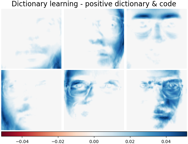
Dictionary learning - positive dictionary & code#
Also below are the results if the dictionary values and coding coefficients are positively constrained.
dict_pos_estimator = decomposition.MiniBatchDictionaryLearning(
    n_components=n_components,
    alpha=0.1,
    max_iter=50,
    batch_size=3,
    fit_algorithm="cd",
    random_state=rng,
    positive_dict=True,
    positive_code=True,
)
dict_pos_estimator.fit(faces_centered)
plot_gallery(
    "Dictionary learning - positive dictionary & code",
    dict_pos_estimator.components_[:n_components],
    cmap=plt.cm.RdBu,
)
/home/circleci/project/sklearn/linear_model/_coordinate_descent.py:825: ConvergenceWarning: Objective did not converge. You might want to increase the number of iterations, check the scale of the features or consider increasing regularisation. Duality gap: 4.768372e-06, tolerance: 5.226e-07
  model = cd_fast.enet_coordinate_descent_gram(
/home/circleci/project/sklearn/linear_model/_coordinate_descent.py:825: ConvergenceWarning: Objective did not converge. You might want to increase the number of iterations, check the scale of the features or consider increasing regularisation. Duality gap: 3.814697e-06, tolerance: 8.048e-07
  model = cd_fast.enet_coordinate_descent_gram(
/home/circleci/project/sklearn/linear_model/_coordinate_descent.py:825: ConvergenceWarning: Objective did not converge. You might want to increase the number of iterations, check the scale of the features or consider increasing regularisation. Duality gap: 5.722046e-06, tolerance: 4.417e-07
  model = cd_fast.enet_coordinate_descent_gram(
/home/circleci/project/sklearn/linear_model/_coordinate_descent.py:825: ConvergenceWarning: Objective did not converge. You might want to increase the number of iterations, check the scale of the features or consider increasing regularisation. Duality gap: 1.907349e-06, tolerance: 5.318e-07
  model = cd_fast.enet_coordinate_descent_gram(
/home/circleci/project/sklearn/linear_model/_coordinate_descent.py:825: ConvergenceWarning: Objective did not converge. You might want to increase the number of iterations, check the scale of the features or consider increasing regularisation. Duality gap: 1.907349e-06, tolerance: 3.365e-07
  model = cd_fast.enet_coordinate_descent_gram(
/home/circleci/project/sklearn/linear_model/_coordinate_descent.py:825: ConvergenceWarning: Objective did not converge. You might want to increase the number of iterations, check the scale of the features or consider increasing regularisation. Duality gap: 1.907349e-06, tolerance: 6.049e-07
  model = cd_fast.enet_coordinate_descent_gram(
/home/circleci/project/sklearn/linear_model/_coordinate_descent.py:825: ConvergenceWarning: Objective did not converge. You might want to increase the number of iterations, check the scale of the features or consider increasing regularisation. Duality gap: 7.629395e-06, tolerance: 8.307e-07
  model = cd_fast.enet_coordinate_descent_gram(
/home/circleci/project/sklearn/linear_model/_coordinate_descent.py:825: ConvergenceWarning: Objective did not converge. You might want to increase the number of iterations, check the scale of the features or consider increasing regularisation. Duality gap: 1.907349e-06, tolerance: 6.041e-07
  model = cd_fast.enet_coordinate_descent_gram(
/home/circleci/project/sklearn/linear_model/_coordinate_descent.py:825: ConvergenceWarning: Objective did not converge. You might want to increase the number of iterations, check the scale of the features or consider increasing regularisation. Duality gap: 7.629395e-06, tolerance: 1.163e-06
  model = cd_fast.enet_coordinate_descent_gram(
/home/circleci/project/sklearn/linear_model/_coordinate_descent.py:825: ConvergenceWarning: Objective did not converge. You might want to increase the number of iterations, check the scale of the features or consider increasing regularisation. Duality gap: 3.814697e-06, tolerance: 9.421e-07
  model = cd_fast.enet_coordinate_descent_gram(
/home/circleci/project/sklearn/linear_model/_coordinate_descent.py:825: ConvergenceWarning: Objective did not converge. You might want to increase the number of iterations, check the scale of the features or consider increasing regularisation. Duality gap: 1.907349e-06, tolerance: 3.033e-07
  model = cd_fast.enet_coordinate_descent_gram(
/home/circleci/project/sklearn/linear_model/_coordinate_descent.py:825: ConvergenceWarning: Objective did not converge. You might want to increase the number of iterations, check the scale of the features or consider increasing regularisation. Duality gap: 1.907349e-06, tolerance: 3.795e-07
  model = cd_fast.enet_coordinate_descent_gram(
/home/circleci/project/sklearn/linear_model/_coordinate_descent.py:825: ConvergenceWarning: Objective did not converge. You might want to increase the number of iterations, check the scale of the features or consider increasing regularisation. Duality gap: 1.907349e-06, tolerance: 4.180e-07
  model = cd_fast.enet_coordinate_descent_gram(
/home/circleci/project/sklearn/linear_model/_coordinate_descent.py:825: ConvergenceWarning: Objective did not converge. You might want to increase the number of iterations, check the scale of the features or consider increasing regularisation. Duality gap: 5.722046e-06, tolerance: 6.907e-07
  model = cd_fast.enet_coordinate_descent_gram(
/home/circleci/project/sklearn/linear_model/_coordinate_descent.py:825: ConvergenceWarning: Objective did not converge. You might want to increase the number of iterations, check the scale of the features or consider increasing regularisation. Duality gap: 7.629395e-06, tolerance: 7.474e-07
  model = cd_fast.enet_coordinate_descent_gram(
/home/circleci/project/sklearn/linear_model/_coordinate_descent.py:825: ConvergenceWarning: Objective did not converge. You might want to increase the number of iterations, check the scale of the features or consider increasing regularisation. Duality gap: 1.907349e-06, tolerance: 5.948e-07
  model = cd_fast.enet_coordinate_descent_gram(
/home/circleci/project/sklearn/linear_model/_coordinate_descent.py:825: ConvergenceWarning: Objective did not converge. You might want to increase the number of iterations, check the scale of the features or consider increasing regularisation. Duality gap: 5.722046e-06, tolerance: 5.981e-07
  model = cd_fast.enet_coordinate_descent_gram(
/home/circleci/project/sklearn/linear_model/_coordinate_descent.py:825: ConvergenceWarning: Objective did not converge. You might want to increase the number of iterations, check the scale of the features or consider increasing regularisation. Duality gap: 1.907349e-06, tolerance: 4.631e-07
  model = cd_fast.enet_coordinate_descent_gram(
/home/circleci/project/sklearn/linear_model/_coordinate_descent.py:825: ConvergenceWarning: Objective did not converge. You might want to increase the number of iterations, check the scale of the features or consider increasing regularisation. Duality gap: 3.814697e-06, tolerance: 7.320e-07
  model = cd_fast.enet_coordinate_descent_gram(
/home/circleci/project/sklearn/linear_model/_coordinate_descent.py:825: ConvergenceWarning: Objective did not converge. You might want to increase the number of iterations, check the scale of the features or consider increasing regularisation. Duality gap: 5.722046e-06, tolerance: 5.125e-07
  model = cd_fast.enet_coordinate_descent_gram(
/home/circleci/project/sklearn/linear_model/_coordinate_descent.py:825: ConvergenceWarning: Objective did not converge. You might want to increase the number of iterations, check the scale of the features or consider increasing regularisation. Duality gap: 1.907349e-06, tolerance: 6.737e-07
  model = cd_fast.enet_coordinate_descent_gram(
/home/circleci/project/sklearn/linear_model/_coordinate_descent.py:825: ConvergenceWarning: Objective did not converge. You might want to increase the number of iterations, check the scale of the features or consider increasing regularisation. Duality gap: 7.629395e-06, tolerance: 8.388e-07
  model = cd_fast.enet_coordinate_descent_gram(
/home/circleci/project/sklearn/linear_model/_coordinate_descent.py:825: ConvergenceWarning: Objective did not converge. You might want to increase the number of iterations, check the scale of the features or consider increasing regularisation. Duality gap: 1.907349e-06, tolerance: 4.763e-07
  model = cd_fast.enet_coordinate_descent_gram(
/home/circleci/project/sklearn/linear_model/_coordinate_descent.py:825: ConvergenceWarning: Objective did not converge. You might want to increase the number of iterations, check the scale of the features or consider increasing regularisation. Duality gap: 1.907349e-06, tolerance: 5.547e-07
  model = cd_fast.enet_coordinate_descent_gram(
/home/circleci/project/sklearn/linear_model/_coordinate_descent.py:825: ConvergenceWarning: Objective did not converge. You might want to increase the number of iterations, check the scale of the features or consider increasing regularisation. Duality gap: 1.907349e-06, tolerance: 5.956e-07
  model = cd_fast.enet_coordinate_descent_gram(
/home/circleci/project/sklearn/linear_model/_coordinate_descent.py:825: ConvergenceWarning: Objective did not converge. You might want to increase the number of iterations, check the scale of the features or consider increasing regularisation. Duality gap: 3.814697e-06, tolerance: 9.119e-07
  model = cd_fast.enet_coordinate_descent_gram(
/home/circleci/project/sklearn/linear_model/_coordinate_descent.py:825: ConvergenceWarning: Objective did not converge. You might want to increase the number of iterations, check the scale of the features or consider increasing regularisation. Duality gap: 3.814697e-06, tolerance: 5.047e-07
  model = cd_fast.enet_coordinate_descent_gram(
/home/circleci/project/sklearn/linear_model/_coordinate_descent.py:825: ConvergenceWarning: Objective did not converge. You might want to increase the number of iterations, check the scale of the features or consider increasing regularisation. Duality gap: 1.907349e-06, tolerance: 4.681e-07
  model = cd_fast.enet_coordinate_descent_gram(
/home/circleci/project/sklearn/linear_model/_coordinate_descent.py:825: ConvergenceWarning: Objective did not converge. You might want to increase the number of iterations, check the scale of the features or consider increasing regularisation. Duality gap: 3.814697e-06, tolerance: 6.841e-07
  model = cd_fast.enet_coordinate_descent_gram(
/home/circleci/project/sklearn/linear_model/_coordinate_descent.py:825: ConvergenceWarning: Objective did not converge. You might want to increase the number of iterations, check the scale of the features or consider increasing regularisation. Duality gap: 9.536743e-07, tolerance: 2.732e-07
  model = cd_fast.enet_coordinate_descent_gram(
/home/circleci/project/sklearn/linear_model/_coordinate_descent.py:825: ConvergenceWarning: Objective did not converge. You might want to increase the number of iterations, check the scale of the features or consider increasing regularisation. Duality gap: 1.907349e-06, tolerance: 3.357e-07
  model = cd_fast.enet_coordinate_descent_gram(
/home/circleci/project/sklearn/linear_model/_coordinate_descent.py:825: ConvergenceWarning: Objective did not converge. You might want to increase the number of iterations, check the scale of the features or consider increasing regularisation. Duality gap: 1.907349e-06, tolerance: 4.374e-07
  model = cd_fast.enet_coordinate_descent_gram(
/home/circleci/project/sklearn/linear_model/_coordinate_descent.py:825: ConvergenceWarning: Objective did not converge. You might want to increase the number of iterations, check the scale of the features or consider increasing regularisation. Duality gap: 7.629395e-06, tolerance: 7.240e-07
  model = cd_fast.enet_coordinate_descent_gram(
/home/circleci/project/sklearn/linear_model/_coordinate_descent.py:825: ConvergenceWarning: Objective did not converge. You might want to increase the number of iterations, check the scale of the features or consider increasing regularisation. Duality gap: 1.907349e-06, tolerance: 5.870e-07
  model = cd_fast.enet_coordinate_descent_gram(
/home/circleci/project/sklearn/linear_model/_coordinate_descent.py:825: ConvergenceWarning: Objective did not converge. You might want to increase the number of iterations, check the scale of the features or consider increasing regularisation. Duality gap: 3.814697e-06, tolerance: 4.510e-07
  model = cd_fast.enet_coordinate_descent_gram(
/home/circleci/project/sklearn/linear_model/_coordinate_descent.py:825: ConvergenceWarning: Objective did not converge. You might want to increase the number of iterations, check the scale of the features or consider increasing regularisation. Duality gap: 7.629395e-06, tolerance: 8.743e-07
  model = cd_fast.enet_coordinate_descent_gram(
/home/circleci/project/sklearn/linear_model/_coordinate_descent.py:825: ConvergenceWarning: Objective did not converge. You might want to increase the number of iterations, check the scale of the features or consider increasing regularisation. Duality gap: 3.814697e-06, tolerance: 8.788e-07
  model = cd_fast.enet_coordinate_descent_gram(
/home/circleci/project/sklearn/linear_model/_coordinate_descent.py:825: ConvergenceWarning: Objective did not converge. You might want to increase the number of iterations, check the scale of the features or consider increasing regularisation. Duality gap: 3.814697e-06, tolerance: 3.096e-07
  model = cd_fast.enet_coordinate_descent_gram(
/home/circleci/project/sklearn/linear_model/_coordinate_descent.py:825: ConvergenceWarning: Objective did not converge. You might want to increase the number of iterations, check the scale of the features or consider increasing regularisation. Duality gap: 1.907349e-06, tolerance: 6.725e-07
  model = cd_fast.enet_coordinate_descent_gram(
/home/circleci/project/sklearn/linear_model/_coordinate_descent.py:825: ConvergenceWarning: Objective did not converge. You might want to increase the number of iterations, check the scale of the features or consider increasing regularisation. Duality gap: 1.907349e-06, tolerance: 4.625e-07
  model = cd_fast.enet_coordinate_descent_gram(
/home/circleci/project/sklearn/linear_model/_coordinate_descent.py:825: ConvergenceWarning: Objective did not converge. You might want to increase the number of iterations, check the scale of the features or consider increasing regularisation. Duality gap: 9.536743e-07, tolerance: 3.092e-07
  model = cd_fast.enet_coordinate_descent_gram(
/home/circleci/project/sklearn/linear_model/_coordinate_descent.py:825: ConvergenceWarning: Objective did not converge. You might want to increase the number of iterations, check the scale of the features or consider increasing regularisation. Duality gap: 3.814697e-06, tolerance: 7.140e-07
  model = cd_fast.enet_coordinate_descent_gram(
/home/circleci/project/sklearn/linear_model/_coordinate_descent.py:825: ConvergenceWarning: Objective did not converge. You might want to increase the number of iterations, check the scale of the features or consider increasing regularisation. Duality gap: 3.814697e-06, tolerance: 3.956e-07
  model = cd_fast.enet_coordinate_descent_gram(
/home/circleci/project/sklearn/linear_model/_coordinate_descent.py:825: ConvergenceWarning: Objective did not converge. You might want to increase the number of iterations, check the scale of the features or consider increasing regularisation. Duality gap: 7.629395e-06, tolerance: 7.643e-07
  model = cd_fast.enet_coordinate_descent_gram(
/home/circleci/project/sklearn/linear_model/_coordinate_descent.py:825: ConvergenceWarning: Objective did not converge. You might want to increase the number of iterations, check the scale of the features or consider increasing regularisation. Duality gap: 3.814697e-06, tolerance: 6.651e-07
  model = cd_fast.enet_coordinate_descent_gram(
/home/circleci/project/sklearn/linear_model/_coordinate_descent.py:825: ConvergenceWarning: Objective did not converge. You might want to increase the number of iterations, check the scale of the features or consider increasing regularisation. Duality gap: 3.814697e-06, tolerance: 4.669e-07
  model = cd_fast.enet_coordinate_descent_gram(
/home/circleci/project/sklearn/linear_model/_coordinate_descent.py:825: ConvergenceWarning: Objective did not converge. You might want to increase the number of iterations, check the scale of the features or consider increasing regularisation. Duality gap: 3.814697e-06, tolerance: 9.390e-07
  model = cd_fast.enet_coordinate_descent_gram(
/home/circleci/project/sklearn/linear_model/_coordinate_descent.py:825: ConvergenceWarning: Objective did not converge. You might want to increase the number of iterations, check the scale of the features or consider increasing regularisation. Duality gap: 2.861023e-06, tolerance: 2.994e-07
  model = cd_fast.enet_coordinate_descent_gram(
/home/circleci/project/sklearn/linear_model/_coordinate_descent.py:825: ConvergenceWarning: Objective did not converge. You might want to increase the number of iterations, check the scale of the features or consider increasing regularisation. Duality gap: 1.907349e-06, tolerance: 6.572e-07
  model = cd_fast.enet_coordinate_descent_gram(
/home/circleci/project/sklearn/linear_model/_coordinate_descent.py:825: ConvergenceWarning: Objective did not converge. You might want to increase the number of iterations, check the scale of the features or consider increasing regularisation. Duality gap: 3.814697e-06, tolerance: 1.035e-06
  model = cd_fast.enet_coordinate_descent_gram(
/home/circleci/project/sklearn/linear_model/_coordinate_descent.py:825: ConvergenceWarning: Objective did not converge. You might want to increase the number of iterations, check the scale of the features or consider increasing regularisation. Duality gap: 1.907349e-06, tolerance: 5.379e-07
  model = cd_fast.enet_coordinate_descent_gram(
/home/circleci/project/sklearn/linear_model/_coordinate_descent.py:825: ConvergenceWarning: Objective did not converge. You might want to increase the number of iterations, check the scale of the features or consider increasing regularisation. Duality gap: 9.536743e-07, tolerance: 1.841e-07
  model = cd_fast.enet_coordinate_descent_gram(
/home/circleci/project/sklearn/linear_model/_coordinate_descent.py:825: ConvergenceWarning: Objective did not converge. You might want to increase the number of iterations, check the scale of the features or consider increasing regularisation. Duality gap: 1.907349e-06, tolerance: 6.932e-07
  model = cd_fast.enet_coordinate_descent_gram(
/home/circleci/project/sklearn/linear_model/_coordinate_descent.py:825: ConvergenceWarning: Objective did not converge. You might want to increase the number of iterations, check the scale of the features or consider increasing regularisation. Duality gap: 3.814697e-06, tolerance: 9.130e-07
  model = cd_fast.enet_coordinate_descent_gram(
/home/circleci/project/sklearn/linear_model/_coordinate_descent.py:825: ConvergenceWarning: Objective did not converge. You might want to increase the number of iterations, check the scale of the features or consider increasing regularisation. Duality gap: 7.629395e-06, tolerance: 8.545e-07
  model = cd_fast.enet_coordinate_descent_gram(
/home/circleci/project/sklearn/linear_model/_coordinate_descent.py:825: ConvergenceWarning: Objective did not converge. You might want to increase the number of iterations, check the scale of the features or consider increasing regularisation. Duality gap: 1.907349e-06, tolerance: 6.543e-07
  model = cd_fast.enet_coordinate_descent_gram(
/home/circleci/project/sklearn/linear_model/_coordinate_descent.py:825: ConvergenceWarning: Objective did not converge. You might want to increase the number of iterations, check the scale of the features or consider increasing regularisation. Duality gap: 3.814697e-06, tolerance: 8.678e-07
  model = cd_fast.enet_coordinate_descent_gram(
/home/circleci/project/sklearn/linear_model/_coordinate_descent.py:825: ConvergenceWarning: Objective did not converge. You might want to increase the number of iterations, check the scale of the features or consider increasing regularisation. Duality gap: 1.907349e-06, tolerance: 4.980e-07
  model = cd_fast.enet_coordinate_descent_gram(
/home/circleci/project/sklearn/linear_model/_coordinate_descent.py:825: ConvergenceWarning: Objective did not converge. You might want to increase the number of iterations, check the scale of the features or consider increasing regularisation. Duality gap: 7.629395e-06, tolerance: 9.927e-07
  model = cd_fast.enet_coordinate_descent_gram(
/home/circleci/project/sklearn/linear_model/_coordinate_descent.py:825: ConvergenceWarning: Objective did not converge. You might want to increase the number of iterations, check the scale of the features or consider increasing regularisation. Duality gap: 1.907349e-06, tolerance: 5.747e-07
  model = cd_fast.enet_coordinate_descent_gram(
/home/circleci/project/sklearn/linear_model/_coordinate_descent.py:825: ConvergenceWarning: Objective did not converge. You might want to increase the number of iterations, check the scale of the features or consider increasing regularisation. Duality gap: 9.536743e-07, tolerance: 2.861e-07
  model = cd_fast.enet_coordinate_descent_gram(
/home/circleci/project/sklearn/linear_model/_coordinate_descent.py:825: ConvergenceWarning: Objective did not converge. You might want to increase the number of iterations, check the scale of the features or consider increasing regularisation. Duality gap: 1.907349e-06, tolerance: 5.069e-07
  model = cd_fast.enet_coordinate_descent_gram(
/home/circleci/project/sklearn/linear_model/_coordinate_descent.py:825: ConvergenceWarning: Objective did not converge. You might want to increase the number of iterations, check the scale of the features or consider increasing regularisation. Duality gap: 1.907349e-06, tolerance: 4.199e-07
  model = cd_fast.enet_coordinate_descent_gram(
/home/circleci/project/sklearn/linear_model/_coordinate_descent.py:825: ConvergenceWarning: Objective did not converge. You might want to increase the number of iterations, check the scale of the features or consider increasing regularisation. Duality gap: 1.907349e-06, tolerance: 5.710e-07
  model = cd_fast.enet_coordinate_descent_gram(
/home/circleci/project/sklearn/linear_model/_coordinate_descent.py:825: ConvergenceWarning: Objective did not converge. You might want to increase the number of iterations, check the scale of the features or consider increasing regularisation. Duality gap: 3.814697e-06, tolerance: 1.654e-06
  model = cd_fast.enet_coordinate_descent_gram(
/home/circleci/project/sklearn/linear_model/_coordinate_descent.py:825: ConvergenceWarning: Objective did not converge. You might want to increase the number of iterations, check the scale of the features or consider increasing regularisation. Duality gap: 1.907349e-06, tolerance: 5.176e-07
  model = cd_fast.enet_coordinate_descent_gram(
/home/circleci/project/sklearn/linear_model/_coordinate_descent.py:825: ConvergenceWarning: Objective did not converge. You might want to increase the number of iterations, check the scale of the features or consider increasing regularisation. Duality gap: 3.814697e-06, tolerance: 5.575e-07
  model = cd_fast.enet_coordinate_descent_gram(
/home/circleci/project/sklearn/linear_model/_coordinate_descent.py:825: ConvergenceWarning: Objective did not converge. You might want to increase the number of iterations, check the scale of the features or consider increasing regularisation. Duality gap: 1.907349e-06, tolerance: 3.308e-07
  model = cd_fast.enet_coordinate_descent_gram(
/home/circleci/project/sklearn/linear_model/_coordinate_descent.py:825: ConvergenceWarning: Objective did not converge. You might want to increase the number of iterations, check the scale of the features or consider increasing regularisation. Duality gap: 1.907349e-06, tolerance: 7.094e-07
  model = cd_fast.enet_coordinate_descent_gram(
/home/circleci/project/sklearn/linear_model/_coordinate_descent.py:825: ConvergenceWarning: Objective did not converge. You might want to increase the number of iterations, check the scale of the features or consider increasing regularisation. Duality gap: 1.907349e-06, tolerance: 5.350e-07
  model = cd_fast.enet_coordinate_descent_gram(
/home/circleci/project/sklearn/linear_model/_coordinate_descent.py:825: ConvergenceWarning: Objective did not converge. You might want to increase the number of iterations, check the scale of the features or consider increasing regularisation. Duality gap: 1.907349e-06, tolerance: 4.340e-07
  model = cd_fast.enet_coordinate_descent_gram(
/home/circleci/project/sklearn/linear_model/_coordinate_descent.py:825: ConvergenceWarning: Objective did not converge. You might want to increase the number of iterations, check the scale of the features or consider increasing regularisation. Duality gap: 9.536743e-07, tolerance: 2.944e-07
  model = cd_fast.enet_coordinate_descent_gram(
/home/circleci/project/sklearn/linear_model/_coordinate_descent.py:825: ConvergenceWarning: Objective did not converge. You might want to increase the number of iterations, check the scale of the features or consider increasing regularisation. Duality gap: 3.814697e-06, tolerance: 4.926e-07
  model = cd_fast.enet_coordinate_descent_gram(
/home/circleci/project/sklearn/linear_model/_coordinate_descent.py:825: ConvergenceWarning: Objective did not converge. You might want to increase the number of iterations, check the scale of the features or consider increasing regularisation. Duality gap: 7.629395e-06, tolerance: 7.919e-07
  model = cd_fast.enet_coordinate_descent_gram(
/home/circleci/project/sklearn/linear_model/_coordinate_descent.py:825: ConvergenceWarning: Objective did not converge. You might want to increase the number of iterations, check the scale of the features or consider increasing regularisation. Duality gap: 5.722046e-06, tolerance: 4.869e-07
  model = cd_fast.enet_coordinate_descent_gram(
/home/circleci/project/sklearn/linear_model/_coordinate_descent.py:825: ConvergenceWarning: Objective did not converge. You might want to increase the number of iterations, check the scale of the features or consider increasing regularisation. Duality gap: 1.907349e-06, tolerance: 4.134e-07
  model = cd_fast.enet_coordinate_descent_gram(
/home/circleci/project/sklearn/linear_model/_coordinate_descent.py:825: ConvergenceWarning: Objective did not converge. You might want to increase the number of iterations, check the scale of the features or consider increasing regularisation. Duality gap: 1.907349e-06, tolerance: 2.367e-07
  model = cd_fast.enet_coordinate_descent_gram(
/home/circleci/project/sklearn/linear_model/_coordinate_descent.py:825: ConvergenceWarning: Objective did not converge. You might want to increase the number of iterations, check the scale of the features or consider increasing regularisation. Duality gap: 3.814697e-06, tolerance: 7.128e-07
  model = cd_fast.enet_coordinate_descent_gram(
/home/circleci/project/sklearn/linear_model/_coordinate_descent.py:825: ConvergenceWarning: Objective did not converge. You might want to increase the number of iterations, check the scale of the features or consider increasing regularisation. Duality gap: 1.907349e-06, tolerance: 3.557e-07
  model = cd_fast.enet_coordinate_descent_gram(
/home/circleci/project/sklearn/linear_model/_coordinate_descent.py:825: ConvergenceWarning: Objective did not converge. You might want to increase the number of iterations, check the scale of the features or consider increasing regularisation. Duality gap: 3.814697e-06, tolerance: 6.564e-07
  model = cd_fast.enet_coordinate_descent_gram(
/home/circleci/project/sklearn/linear_model/_coordinate_descent.py:825: ConvergenceWarning: Objective did not converge. You might want to increase the number of iterations, check the scale of the features or consider increasing regularisation. Duality gap: 1.907349e-06, tolerance: 3.746e-07
  model = cd_fast.enet_coordinate_descent_gram(
/home/circleci/project/sklearn/linear_model/_coordinate_descent.py:825: ConvergenceWarning: Objective did not converge. You might want to increase the number of iterations, check the scale of the features or consider increasing regularisation. Duality gap: 3.814697e-06, tolerance: 7.491e-07
  model = cd_fast.enet_coordinate_descent_gram(
/home/circleci/project/sklearn/linear_model/_coordinate_descent.py:825: ConvergenceWarning: Objective did not converge. You might want to increase the number of iterations, check the scale of the features or consider increasing regularisation. Duality gap: 3.814697e-06, tolerance: 6.478e-07
  model = cd_fast.enet_coordinate_descent_gram(
/home/circleci/project/sklearn/linear_model/_coordinate_descent.py:825: ConvergenceWarning: Objective did not converge. You might want to increase the number of iterations, check the scale of the features or consider increasing regularisation. Duality gap: 1.907349e-06, tolerance: 7.690e-07
  model = cd_fast.enet_coordinate_descent_gram(
/home/circleci/project/sklearn/linear_model/_coordinate_descent.py:825: ConvergenceWarning: Objective did not converge. You might want to increase the number of iterations, check the scale of the features or consider increasing regularisation. Duality gap: 3.814697e-06, tolerance: 8.224e-07
  model = cd_fast.enet_coordinate_descent_gram(
/home/circleci/project/sklearn/linear_model/_coordinate_descent.py:825: ConvergenceWarning: Objective did not converge. You might want to increase the number of iterations, check the scale of the features or consider increasing regularisation. Duality gap: 3.814697e-06, tolerance: 8.168e-07
  model = cd_fast.enet_coordinate_descent_gram(
/home/circleci/project/sklearn/linear_model/_coordinate_descent.py:825: ConvergenceWarning: Objective did not converge. You might want to increase the number of iterations, check the scale of the features or consider increasing regularisation. Duality gap: 1.907349e-06, tolerance: 5.028e-07
  model = cd_fast.enet_coordinate_descent_gram(
/home/circleci/project/sklearn/linear_model/_coordinate_descent.py:825: ConvergenceWarning: Objective did not converge. You might want to increase the number of iterations, check the scale of the features or consider increasing regularisation. Duality gap: 3.814697e-06, tolerance: 6.287e-07
  model = cd_fast.enet_coordinate_descent_gram(
/home/circleci/project/sklearn/linear_model/_coordinate_descent.py:825: ConvergenceWarning: Objective did not converge. You might want to increase the number of iterations, check the scale of the features or consider increasing regularisation. Duality gap: 5.722046e-06, tolerance: 4.778e-07
  model = cd_fast.enet_coordinate_descent_gram(
/home/circleci/project/sklearn/linear_model/_coordinate_descent.py:825: ConvergenceWarning: Objective did not converge. You might want to increase the number of iterations, check the scale of the features or consider increasing regularisation. Duality gap: 5.722046e-06, tolerance: 9.354e-07
  model = cd_fast.enet_coordinate_descent_gram(
/home/circleci/project/sklearn/linear_model/_coordinate_descent.py:825: ConvergenceWarning: Objective did not converge. You might want to increase the number of iterations, check the scale of the features or consider increasing regularisation. Duality gap: 3.814697e-06, tolerance: 6.349e-07
  model = cd_fast.enet_coordinate_descent_gram(
/home/circleci/project/sklearn/linear_model/_coordinate_descent.py:825: ConvergenceWarning: Objective did not converge. You might want to increase the number of iterations, check the scale of the features or consider increasing regularisation. Duality gap: 3.814697e-06, tolerance: 6.518e-07
  model = cd_fast.enet_coordinate_descent_gram(
/home/circleci/project/sklearn/linear_model/_coordinate_descent.py:825: ConvergenceWarning: Objective did not converge. You might want to increase the number of iterations, check the scale of the features or consider increasing regularisation. Duality gap: 3.814697e-06, tolerance: 6.309e-07
  model = cd_fast.enet_coordinate_descent_gram(
/home/circleci/project/sklearn/linear_model/_coordinate_descent.py:825: ConvergenceWarning: Objective did not converge. You might want to increase the number of iterations, check the scale of the features or consider increasing regularisation. Duality gap: 2.861023e-06, tolerance: 3.306e-07
  model = cd_fast.enet_coordinate_descent_gram(
/home/circleci/project/sklearn/linear_model/_coordinate_descent.py:825: ConvergenceWarning: Objective did not converge. You might want to increase the number of iterations, check the scale of the features or consider increasing regularisation. Duality gap: 1.907349e-06, tolerance: 7.107e-07
  model = cd_fast.enet_coordinate_descent_gram(
/home/circleci/project/sklearn/linear_model/_coordinate_descent.py:825: ConvergenceWarning: Objective did not converge. You might want to increase the number of iterations, check the scale of the features or consider increasing regularisation. Duality gap: 1.907349e-06, tolerance: 6.201e-07
  model = cd_fast.enet_coordinate_descent_gram(
/home/circleci/project/sklearn/linear_model/_coordinate_descent.py:825: ConvergenceWarning: Objective did not converge. You might want to increase the number of iterations, check the scale of the features or consider increasing regularisation. Duality gap: 1.907349e-06, tolerance: 6.383e-07
  model = cd_fast.enet_coordinate_descent_gram(
/home/circleci/project/sklearn/linear_model/_coordinate_descent.py:825: ConvergenceWarning: Objective did not converge. You might want to increase the number of iterations, check the scale of the features or consider increasing regularisation. Duality gap: 3.814697e-06, tolerance: 4.301e-07
  model = cd_fast.enet_coordinate_descent_gram(
/home/circleci/project/sklearn/linear_model/_coordinate_descent.py:825: ConvergenceWarning: Objective did not converge. You might want to increase the number of iterations, check the scale of the features or consider increasing regularisation. Duality gap: 3.814697e-06, tolerance: 4.828e-07
  model = cd_fast.enet_coordinate_descent_gram(
/home/circleci/project/sklearn/linear_model/_coordinate_descent.py:825: ConvergenceWarning: Objective did not converge. You might want to increase the number of iterations, check the scale of the features or consider increasing regularisation. Duality gap: 3.814697e-06, tolerance: 8.233e-07
  model = cd_fast.enet_coordinate_descent_gram(
/home/circleci/project/sklearn/linear_model/_coordinate_descent.py:825: ConvergenceWarning: Objective did not converge. You might want to increase the number of iterations, check the scale of the features or consider increasing regularisation. Duality gap: 3.814697e-06, tolerance: 8.004e-07
  model = cd_fast.enet_coordinate_descent_gram(
/home/circleci/project/sklearn/linear_model/_coordinate_descent.py:825: ConvergenceWarning: Objective did not converge. You might want to increase the number of iterations, check the scale of the features or consider increasing regularisation. Duality gap: 1.907349e-06, tolerance: 3.891e-07
  model = cd_fast.enet_coordinate_descent_gram(
/home/circleci/project/sklearn/linear_model/_coordinate_descent.py:825: ConvergenceWarning: Objective did not converge. You might want to increase the number of iterations, check the scale of the features or consider increasing regularisation. Duality gap: 1.907349e-06, tolerance: 3.633e-07
  model = cd_fast.enet_coordinate_descent_gram(
/home/circleci/project/sklearn/linear_model/_coordinate_descent.py:825: ConvergenceWarning: Objective did not converge. You might want to increase the number of iterations, check the scale of the features or consider increasing regularisation. Duality gap: 5.722046e-06, tolerance: 5.658e-07
  model = cd_fast.enet_coordinate_descent_gram(
/home/circleci/project/sklearn/linear_model/_coordinate_descent.py:825: ConvergenceWarning: Objective did not converge. You might want to increase the number of iterations, check the scale of the features or consider increasing regularisation. Duality gap: 9.536743e-07, tolerance: 3.449e-07
  model = cd_fast.enet_coordinate_descent_gram(
/home/circleci/project/sklearn/linear_model/_coordinate_descent.py:825: ConvergenceWarning: Objective did not converge. You might want to increase the number of iterations, check the scale of the features or consider increasing regularisation. Duality gap: 3.814697e-06, tolerance: 7.624e-07
  model = cd_fast.enet_coordinate_descent_gram(
/home/circleci/project/sklearn/linear_model/_coordinate_descent.py:825: ConvergenceWarning: Objective did not converge. You might want to increase the number of iterations, check the scale of the features or consider increasing regularisation. Duality gap: 1.907349e-06, tolerance: 5.098e-07
  model = cd_fast.enet_coordinate_descent_gram(
/home/circleci/project/sklearn/linear_model/_coordinate_descent.py:825: ConvergenceWarning: Objective did not converge. You might want to increase the number of iterations, check the scale of the features or consider increasing regularisation. Duality gap: 1.907349e-06, tolerance: 7.025e-07
  model = cd_fast.enet_coordinate_descent_gram(
/home/circleci/project/sklearn/linear_model/_coordinate_descent.py:825: ConvergenceWarning: Objective did not converge. You might want to increase the number of iterations, check the scale of the features or consider increasing regularisation. Duality gap: 1.907349e-06, tolerance: 3.901e-07
  model = cd_fast.enet_coordinate_descent_gram(
/home/circleci/project/sklearn/linear_model/_coordinate_descent.py:825: ConvergenceWarning: Objective did not converge. You might want to increase the number of iterations, check the scale of the features or consider increasing regularisation. Duality gap: 3.814697e-06, tolerance: 7.027e-07
  model = cd_fast.enet_coordinate_descent_gram(
/home/circleci/project/sklearn/linear_model/_coordinate_descent.py:825: ConvergenceWarning: Objective did not converge. You might want to increase the number of iterations, check the scale of the features or consider increasing regularisation. Duality gap: 3.814697e-06, tolerance: 4.249e-07
  model = cd_fast.enet_coordinate_descent_gram(
/home/circleci/project/sklearn/linear_model/_coordinate_descent.py:825: ConvergenceWarning: Objective did not converge. You might want to increase the number of iterations, check the scale of the features or consider increasing regularisation. Duality gap: 1.335144e-05, tolerance: 9.957e-07
  model = cd_fast.enet_coordinate_descent_gram(
/home/circleci/project/sklearn/linear_model/_coordinate_descent.py:825: ConvergenceWarning: Objective did not converge. You might want to increase the number of iterations, check the scale of the features or consider increasing regularisation. Duality gap: 1.907349e-06, tolerance: 3.199e-07
  model = cd_fast.enet_coordinate_descent_gram(
/home/circleci/project/sklearn/linear_model/_coordinate_descent.py:825: ConvergenceWarning: Objective did not converge. You might want to increase the number of iterations, check the scale of the features or consider increasing regularisation. Duality gap: 3.814697e-06, tolerance: 6.859e-07
  model = cd_fast.enet_coordinate_descent_gram(
/home/circleci/project/sklearn/linear_model/_coordinate_descent.py:825: ConvergenceWarning: Objective did not converge. You might want to increase the number of iterations, check the scale of the features or consider increasing regularisation. Duality gap: 3.814697e-06, tolerance: 8.329e-07
  model = cd_fast.enet_coordinate_descent_gram(
/home/circleci/project/sklearn/linear_model/_coordinate_descent.py:825: ConvergenceWarning: Objective did not converge. You might want to increase the number of iterations, check the scale of the features or consider increasing regularisation. Duality gap: 1.907349e-06, tolerance: 4.796e-07
  model = cd_fast.enet_coordinate_descent_gram(
/home/circleci/project/sklearn/linear_model/_coordinate_descent.py:825: ConvergenceWarning: Objective did not converge. You might want to increase the number of iterations, check the scale of the features or consider increasing regularisation. Duality gap: 3.814697e-06, tolerance: 5.079e-07
  model = cd_fast.enet_coordinate_descent_gram(
/home/circleci/project/sklearn/linear_model/_coordinate_descent.py:825: ConvergenceWarning: Objective did not converge. You might want to increase the number of iterations, check the scale of the features or consider increasing regularisation. Duality gap: 7.629395e-06, tolerance: 1.918e-06
  model = cd_fast.enet_coordinate_descent_gram(
/home/circleci/project/sklearn/linear_model/_coordinate_descent.py:825: ConvergenceWarning: Objective did not converge. You might want to increase the number of iterations, check the scale of the features or consider increasing regularisation. Duality gap: 9.536743e-06, tolerance: 1.014e-06
  model = cd_fast.enet_coordinate_descent_gram(
/home/circleci/project/sklearn/linear_model/_coordinate_descent.py:825: ConvergenceWarning: Objective did not converge. You might want to increase the number of iterations, check the scale of the features or consider increasing regularisation. Duality gap: 7.629395e-06, tolerance: 1.078e-06
  model = cd_fast.enet_coordinate_descent_gram(
/home/circleci/project/sklearn/linear_model/_coordinate_descent.py:825: ConvergenceWarning: Objective did not converge. You might want to increase the number of iterations, check the scale of the features or consider increasing regularisation. Duality gap: 1.907349e-06, tolerance: 6.657e-07
  model = cd_fast.enet_coordinate_descent_gram(
/home/circleci/project/sklearn/linear_model/_coordinate_descent.py:825: ConvergenceWarning: Objective did not converge. You might want to increase the number of iterations, check the scale of the features or consider increasing regularisation. Duality gap: 7.629395e-06, tolerance: 1.527e-06
  model = cd_fast.enet_coordinate_descent_gram(
/home/circleci/project/sklearn/linear_model/_coordinate_descent.py:825: ConvergenceWarning: Objective did not converge. You might want to increase the number of iterations, check the scale of the features or consider increasing regularisation. Duality gap: 9.536743e-07, tolerance: 2.331e-07
  model = cd_fast.enet_coordinate_descent_gram(
/home/circleci/project/sklearn/linear_model/_coordinate_descent.py:825: ConvergenceWarning: Objective did not converge. You might want to increase the number of iterations, check the scale of the features or consider increasing regularisation. Duality gap: 1.907349e-06, tolerance: 5.793e-07
  model = cd_fast.enet_coordinate_descent_gram(
/home/circleci/project/sklearn/linear_model/_coordinate_descent.py:825: ConvergenceWarning: Objective did not converge. You might want to increase the number of iterations, check the scale of the features or consider increasing regularisation. Duality gap: 1.907349e-06, tolerance: 7.015e-07
  model = cd_fast.enet_coordinate_descent_gram(
/home/circleci/project/sklearn/linear_model/_coordinate_descent.py:825: ConvergenceWarning: Objective did not converge. You might want to increase the number of iterations, check the scale of the features or consider increasing regularisation. Duality gap: 1.907349e-06, tolerance: 6.210e-07
  model = cd_fast.enet_coordinate_descent_gram(
/home/circleci/project/sklearn/linear_model/_coordinate_descent.py:825: ConvergenceWarning: Objective did not converge. You might want to increase the number of iterations, check the scale of the features or consider increasing regularisation. Duality gap: 5.722046e-06, tolerance: 5.070e-07
  model = cd_fast.enet_coordinate_descent_gram(
/home/circleci/project/sklearn/linear_model/_coordinate_descent.py:825: ConvergenceWarning: Objective did not converge. You might want to increase the number of iterations, check the scale of the features or consider increasing regularisation. Duality gap: 1.907349e-06, tolerance: 3.944e-07
  model = cd_fast.enet_coordinate_descent_gram(
/home/circleci/project/sklearn/linear_model/_coordinate_descent.py:825: ConvergenceWarning: Objective did not converge. You might want to increase the number of iterations, check the scale of the features or consider increasing regularisation. Duality gap: 3.814697e-06, tolerance: 4.177e-07
  model = cd_fast.enet_coordinate_descent_gram(
/home/circleci/project/sklearn/linear_model/_coordinate_descent.py:825: ConvergenceWarning: Objective did not converge. You might want to increase the number of iterations, check the scale of the features or consider increasing regularisation. Duality gap: 3.814697e-06, tolerance: 6.055e-07
  model = cd_fast.enet_coordinate_descent_gram(
/home/circleci/project/sklearn/linear_model/_coordinate_descent.py:825: ConvergenceWarning: Objective did not converge. You might want to increase the number of iterations, check the scale of the features or consider increasing regularisation. Duality gap: 1.907349e-06, tolerance: 5.985e-07
  model = cd_fast.enet_coordinate_descent_gram(
/home/circleci/project/sklearn/linear_model/_coordinate_descent.py:825: ConvergenceWarning: Objective did not converge. You might want to increase the number of iterations, check the scale of the features or consider increasing regularisation. Duality gap: 3.814697e-06, tolerance: 6.284e-07
  model = cd_fast.enet_coordinate_descent_gram(
/home/circleci/project/sklearn/linear_model/_coordinate_descent.py:825: ConvergenceWarning: Objective did not converge. You might want to increase the number of iterations, check the scale of the features or consider increasing regularisation. Duality gap: 1.907349e-06, tolerance: 6.342e-07
  model = cd_fast.enet_coordinate_descent_gram(
/home/circleci/project/sklearn/linear_model/_coordinate_descent.py:825: ConvergenceWarning: Objective did not converge. You might want to increase the number of iterations, check the scale of the features or consider increasing regularisation. Duality gap: 5.722046e-06, tolerance: 5.925e-07
  model = cd_fast.enet_coordinate_descent_gram(
Total running time of the script: (0 minutes 7.334 seconds)
Related examples
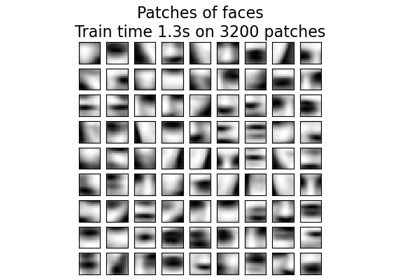
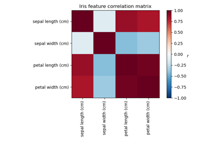
Factor Analysis (with rotation) to visualize patterns
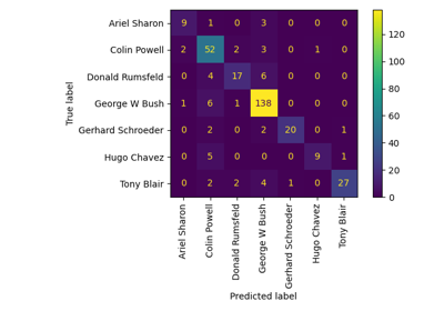
Faces recognition example using eigenfaces and SVMs