Note
Go to the end to download the full example code or to run this example in your browser via JupyterLite or Binder.
Common pitfalls in the interpretation of coefficients of linear models#
In linear models, the target value is modeled as a linear combination of the features (see the Linear Models User Guide section for a description of a set of linear models available in scikit-learn). Coefficients in multiple linear models represent the relationship between the given feature, \(X_i\) and the target, \(y\), assuming that all the other features remain constant (conditional dependence). This is different from plotting \(X_i\) versus \(y\) and fitting a linear relationship: in that case all possible values of the other features are taken into account in the estimation (marginal dependence).
This example will provide some hints in interpreting coefficient in linear models, pointing at problems that arise when either the linear model is not appropriate to describe the dataset, or when features are correlated.
Note
Keep in mind that the features \(X\) and the outcome \(y\) are in general the result of a data generating process that is unknown to us. Machine learning models are trained to approximate the unobserved mathematical function that links \(X\) to \(y\) from sample data. As a result, any interpretation made about a model may not necessarily generalize to the true data generating process. This is especially true when the model is of bad quality or when the sample data is not representative of the population.
We will use data from the “Current Population Survey” from 1985 to predict wage as a function of various features such as experience, age, or education.
# Authors: The scikit-learn developers
# SPDX-License-Identifier: BSD-3-Clause
import matplotlib.pyplot as plt
import numpy as np
import pandas as pd
import scipy as sp
import seaborn as sns
The dataset: wages#
We fetch the data from OpenML.
Note that setting the parameter as_frame to True will retrieve the data
as a pandas dataframe.
from sklearn.datasets import fetch_openml

survey = fetch_openml(data_id=534, as_frame=True)
Then, we identify features X and target y: the column WAGE is our
target variable (i.e. the variable which we want to predict).
X = survey.data[survey.feature_names]
X.describe(include="all")
Note that the dataset contains categorical and numerical variables. We will need to take this into account when preprocessing the dataset thereafter.
X.head()
Our target for prediction: the wage. Wages are described as floating-point number in dollars per hour.
y = survey.target.values.ravel()
survey.target.head()
0    5.10
1    4.95
2    6.67
3    4.00
4    7.50
Name: WAGE, dtype: float64
We split the sample into a train and a test dataset. Only the train dataset will be used in the following exploratory analysis. This is a way to emulate a real situation where predictions are performed on an unknown target, and we don’t want our analysis and decisions to be biased by our knowledge of the test data.
from sklearn.model_selection import train_test_split

X_train, X_test, y_train, y_test = train_test_split(X, y, random_state=42)
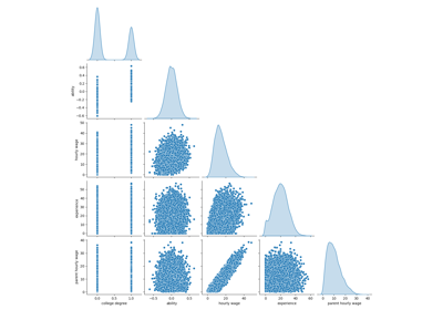
First, let’s get some insights by looking at the variables’ distributions and at the pairwise relationships between them. Only numerical variables will be used. In the following plot, each dot represents a sample.
train_dataset = X_train.copy()
train_dataset.insert(0, "WAGE", y_train)
_ = sns.pairplot(train_dataset, kind="reg", diag_kind="kde")
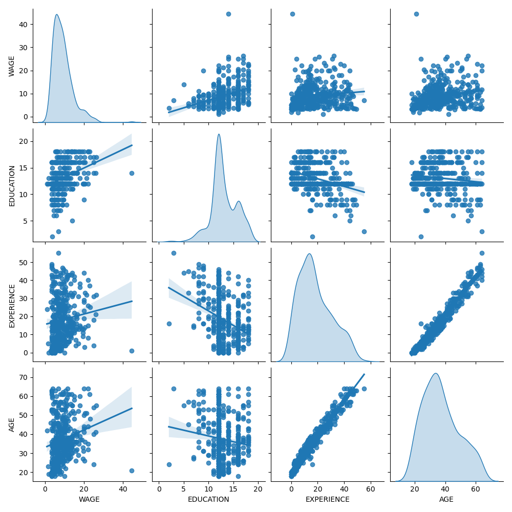
Looking closely at the WAGE distribution reveals that it has a long tail. For this reason, we should take its logarithm to turn it approximately into a normal distribution (linear models such as ridge or lasso work best for a normal distribution of error).
The WAGE is increasing when EDUCATION is increasing. Note that the dependence between WAGE and EDUCATION represented here is a marginal dependence, i.e. it describes the behavior of a specific variable without keeping the others fixed.
Also, the EXPERIENCE and AGE are strongly linearly correlated.
The machine-learning pipeline#
To design our machine-learning pipeline, we first manually check the type of data that we are dealing with:
survey.data.info()
<class 'pandas.DataFrame'>
RangeIndex: 534 entries, 0 to 533
Data columns (total 10 columns):
 #   Column      Non-Null Count  Dtype
---  ------      --------------  -----
 0   EDUCATION   534 non-null    int64
 1   SOUTH       534 non-null    category
 2   SEX         534 non-null    category
 3   EXPERIENCE  534 non-null    int64
 4   UNION       534 non-null    category
 5   AGE         534 non-null    int64
 6   RACE        534 non-null    category
 7   OCCUPATION  534 non-null    category
 8   SECTOR      534 non-null    category
 9   MARR        534 non-null    category
dtypes: category(7), int64(3)
memory usage: 17.3 KB
As seen previously, the dataset contains columns with different data types and we need to apply a specific preprocessing for each data types. In particular categorical variables cannot be included in linear model if not coded as integers first. In addition, to avoid categorical features to be treated as ordered values, we need to one-hot-encode them. Our pre-processor will:
one-hot encode (i.e., generate a column by category) the categorical columns, only for non-binary categorical variables;
as a first approach (we will see after how the normalisation of numerical values will affect our discussion), keep numerical values as they are.
from sklearn.compose import make_column_transformer
from sklearn.preprocessing import OneHotEncoder

categorical_columns = ["RACE", "OCCUPATION", "SECTOR", "MARR", "UNION", "SEX", "SOUTH"]
numerical_columns = ["EDUCATION", "EXPERIENCE", "AGE"]

preprocessor = make_column_transformer(
    (OneHotEncoder(drop="if_binary"), categorical_columns),
    remainder="passthrough",
    verbose_feature_names_out=False,  # avoid to prepend the preprocessor names
)
We use a ridge regressor with a very small regularization to model the logarithm of the WAGE.
from sklearn.compose import TransformedTargetRegressor
from sklearn.linear_model import Ridge
from sklearn.pipeline import make_pipeline

model = make_pipeline(
    preprocessor,
    TransformedTargetRegressor(
        regressor=Ridge(alpha=1e-10), func=np.log10, inverse_func=sp.special.exp10
    ),
)
Processing the dataset#
First, we fit the model.
model.fit(X_train, y_train)
Then we check the performance of the computed model by plotting its predictions against the actual values on the test set, and by computing the median absolute error.
from sklearn.metrics import PredictionErrorDisplay, median_absolute_error

mae_train = median_absolute_error(y_train, model.predict(X_train))
y_pred = model.predict(X_test)
mae_test = median_absolute_error(y_test, y_pred)
scores = {
    "MedAE on training set": f"{mae_train:.2f} $/hour",
    "MedAE on testing set": f"{mae_test:.2f} $/hour",
}
_, ax = plt.subplots(figsize=(5, 5))
display = PredictionErrorDisplay.from_predictions(
    y_test, y_pred, kind="actual_vs_predicted", ax=ax, scatter_kwargs={"alpha": 0.5}
)
ax.set_title("Ridge model, small regularization")
for name, score in scores.items():
    ax.plot([], [], " ", label=f"{name}: {score}")
ax.legend(loc="upper left")
plt.tight_layout()
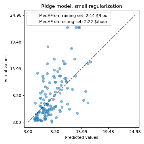
The model learnt is far from being a good model making accurate predictions: this is obvious when looking at the plot above, where good predictions should lie on the black dashed line.
In the following section, we will interpret the coefficients of the model. While we do so, we should keep in mind that any conclusion we draw is about the model that we build, rather than about the true (real-world) generative process of the data.
Interpreting coefficients: scale matters#
First of all, we can take a look to the values of the coefficients of the regressor we have fitted.
feature_names = model[:-1].get_feature_names_out()

coefs = pd.DataFrame(
    model[-1].regressor_.coef_,
    columns=["Coefficients"],
    index=feature_names,
)

coefs
The AGE coefficient is expressed in “dollars/hour per living years” while the EDUCATION one is expressed in “dollars/hour per years of education”. This representation of the coefficients has the benefit of making clear the practical predictions of the model: an increase of \(1\) year in AGE means a decrease of \(0.030867\) dollars/hour, while an increase of \(1\) year in EDUCATION means an increase of \(0.054699\) dollars/hour. On the other hand, categorical variables (as UNION or SEX) are adimensional numbers taking either the value 0 or 1. Their coefficients are expressed in dollars/hour. Then, we cannot compare the magnitude of different coefficients since the features have different natural scales, and hence value ranges, because of their different unit of measure. This is more visible if we plot the coefficients.
coefs.plot.barh(figsize=(9, 7))
plt.title("Ridge model, small regularization")
plt.axvline(x=0, color=".5")
plt.xlabel("Raw coefficient values")
plt.subplots_adjust(left=0.3)
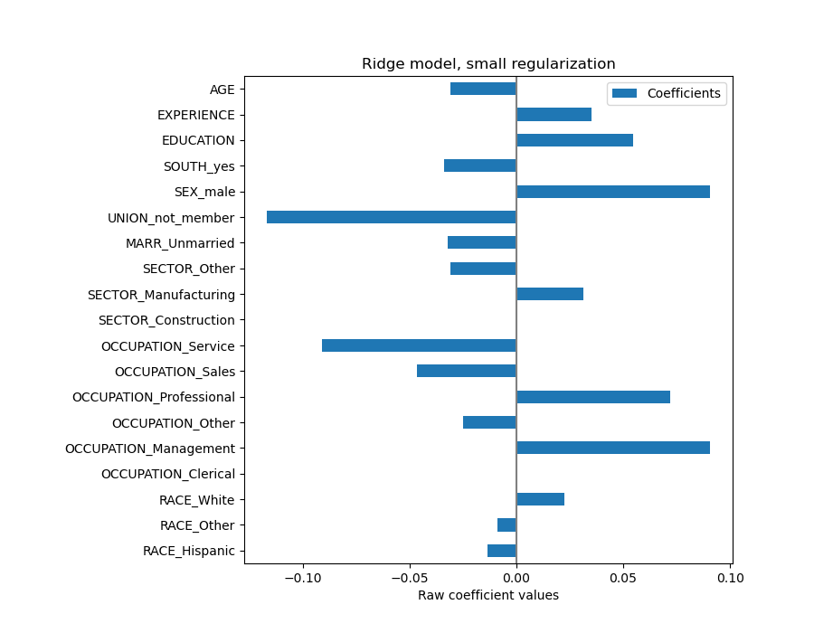
Indeed, from the plot above the most important factor in determining WAGE appears to be the variable UNION, even if our intuition might tell us that variables like EXPERIENCE should have more impact.
Looking at the coefficient plot to gauge feature importance can be misleading as some of them vary on a small scale, while others, like AGE, varies a lot more, several decades.
This is visible if we compare the standard deviations of different features.
X_train_preprocessed = pd.DataFrame(
    model[:-1].transform(X_train), columns=feature_names
)

X_train_preprocessed.std(axis=0).plot.barh(figsize=(9, 7))
plt.title("Feature ranges")
plt.xlabel("Std. dev. of feature values")
plt.subplots_adjust(left=0.3)
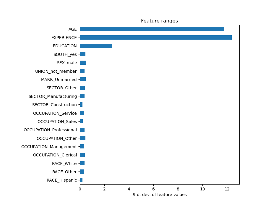
Multiplying the coefficients by the standard deviation of the related feature would reduce all the coefficients to the same unit of measure. As we will see after this is equivalent to normalize numerical variables to their standard deviation, as \(y = \sum{coef_i \times X_i} = \sum{(coef_i \times std_i) \times (X_i / std_i)}\).
In that way, we emphasize that the greater the variance of a feature, the larger the weight of the corresponding coefficient on the output, all else being equal.
coefs = pd.DataFrame(
    model[-1].regressor_.coef_ * X_train_preprocessed.std(axis=0),
    columns=["Coefficient importance"],
    index=feature_names,
)
coefs.plot(kind="barh", figsize=(9, 7))
plt.xlabel("Coefficient values corrected by the feature's std. dev.")
plt.title("Ridge model, small regularization")
plt.axvline(x=0, color=".5")
plt.subplots_adjust(left=0.3)
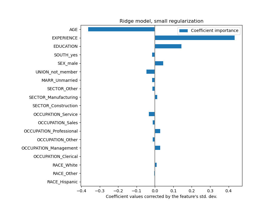
Now that the coefficients have been scaled, we can safely compare them.
Note
Why does the plot above suggest that an increase in age leads to a decrease in wage? Why is the initial pairplot telling the opposite? This difference is the difference between marginal and conditional dependence.
The plot above tells us about dependencies between a specific feature and the target when all other features remain constant, i.e., conditional dependencies. An increase of the AGE will induce a decrease of the WAGE when all other features remain constant. On the contrary, an increase of the EXPERIENCE will induce an increase of the WAGE when all other features remain constant. Also, AGE, EXPERIENCE and EDUCATION are the three variables that most influence the model.
Interpreting coefficients: being cautious about causality#
Linear models are a great tool for measuring statistical association, but we should be cautious when making statements about causality, after all correlation doesn’t always imply causation. This is particularly difficult in the social sciences because the variables we observe only function as proxies for the underlying causal process.
In our particular case we can think of the EDUCATION of an individual as a proxy for their professional aptitude, the real variable we’re interested in but can’t observe. We’d certainly like to think that staying in school for longer would increase technical competency, but it’s also quite possible that causality goes the other way too. That is, those who are technically competent tend to stay in school for longer.
An employer is unlikely to care which case it is (or if it’s a mix of both), as long as they remain convinced that a person with more EDUCATION is better suited for the job, they will be happy to pay out a higher WAGE.
This confounding of effects becomes problematic when thinking about some form of intervention e.g. government subsidies of university degrees or promotional material encouraging individuals to take up higher education. The usefulness of these measures could end up being overstated, especially if the degree of confounding is strong. Our model predicts a \(0.054699\) increase in hourly wage for each year of education. The actual causal effect might be lower because of this confounding.
Checking the variability of the coefficients#
We can check the coefficient variability through cross-validation: it is a form of data perturbation (related to resampling).
If coefficients vary significantly when changing the input dataset their robustness is not guaranteed, and they should probably be interpreted with caution.
from sklearn.model_selection import RepeatedKFold, cross_validate

cv = RepeatedKFold(n_splits=5, n_repeats=5, random_state=0)
cv_model = cross_validate(
    model,
    X,
    y,
    cv=cv,
    return_estimator=True,
    n_jobs=2,
)

coefs = pd.DataFrame(
    [
        est[-1].regressor_.coef_ * est[:-1].transform(X.iloc[train_idx]).std(axis=0)
        for est, (train_idx, _) in zip(cv_model["estimator"], cv.split(X, y))
    ],
    columns=feature_names,
)
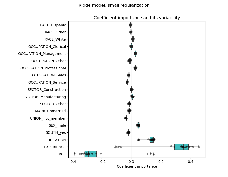
plt.figure(figsize=(9, 7))
sns.stripplot(data=coefs, orient="h", palette="dark:k", alpha=0.5)
sns.boxplot(data=coefs, orient="h", color="cyan", saturation=0.5, whis=10)
plt.axvline(x=0, color=".5")
plt.xlabel("Coefficient importance")
plt.title("Coefficient importance and its variability")
plt.suptitle("Ridge model, small regularization")
plt.subplots_adjust(left=0.3)
The problem of correlated variables#
The AGE and EXPERIENCE coefficients are affected by strong variability which might be due to the collinearity between the 2 features: as AGE and EXPERIENCE vary together in the data, their effect is difficult to tease apart.
To verify this interpretation we plot the variability of the AGE and EXPERIENCE coefficient.
plt.xlabel("Age coefficient")
plt.ylabel("Experience coefficient")
plt.grid(True)
plt.xlim(-0.4, 0.5)
plt.ylim(-0.4, 0.5)
plt.scatter(coefs["AGE"], coefs["EXPERIENCE"])
_ = plt.title("Co-variations of coefficients for AGE and EXPERIENCE across folds")
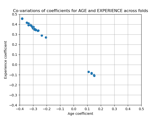
Two regions are populated: when the EXPERIENCE coefficient is positive the AGE one is negative and vice-versa.
To go further we remove one of the two features, AGE, and check what is the impact on the model stability.
column_to_drop = ["AGE"]

cv_model = cross_validate(
    model,
    X.drop(columns=column_to_drop),
    y,
    cv=cv,
    return_estimator=True,
    n_jobs=2,
)

coefs = pd.DataFrame(
    [
        est[-1].regressor_.coef_
        * est[:-1].transform(X.drop(columns=column_to_drop).iloc[train_idx]).std(axis=0)
        for est, (train_idx, _) in zip(cv_model["estimator"], cv.split(X, y))
    ],
    columns=feature_names[:-1],
)
plt.figure(figsize=(9, 7))
sns.stripplot(data=coefs, orient="h", palette="dark:k", alpha=0.5)
sns.boxplot(data=coefs, orient="h", color="cyan", saturation=0.5)
plt.axvline(x=0, color=".5")
plt.title("Coefficient importance and its variability")
plt.xlabel("Coefficient importance")
plt.suptitle("Ridge model, small regularization, AGE dropped")
plt.subplots_adjust(left=0.3)
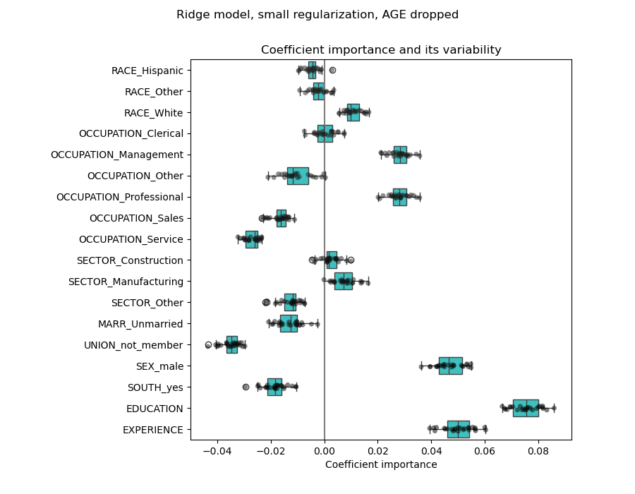
The estimation of the EXPERIENCE coefficient now shows a much reduced variability. EXPERIENCE remains important for all models trained during cross-validation.
Preprocessing numerical variables#
As said above (see “The machine-learning pipeline”), we could also choose to scale numerical values before training the model. This can be useful when we apply a similar amount of regularization to all of them in the ridge. The preprocessor is redefined in order to subtract the mean and scale variables to unit variance.
from sklearn.preprocessing import StandardScaler

preprocessor = make_column_transformer(
    (OneHotEncoder(drop="if_binary"), categorical_columns),
    (StandardScaler(), numerical_columns),
)
The model will stay unchanged.
model = make_pipeline(
    preprocessor,
    TransformedTargetRegressor(
        regressor=Ridge(alpha=1e-10), func=np.log10, inverse_func=sp.special.exp10
    ),
)
model.fit(X_train, y_train)
Again, we check the performance of the computed model using the median absolute error.
mae_train = median_absolute_error(y_train, model.predict(X_train))
y_pred = model.predict(X_test)
mae_test = median_absolute_error(y_test, y_pred)
scores = {
    "MedAE on training set": f"{mae_train:.2f} $/hour",
    "MedAE on testing set": f"{mae_test:.2f} $/hour",
}

_, ax = plt.subplots(figsize=(5, 5))
display = PredictionErrorDisplay.from_predictions(
    y_test, y_pred, kind="actual_vs_predicted", ax=ax, scatter_kwargs={"alpha": 0.5}
)
ax.set_title("Ridge model, small regularization")
for name, score in scores.items():
    ax.plot([], [], " ", label=f"{name}: {score}")
ax.legend(loc="upper left")
plt.tight_layout()

For the coefficient analysis, scaling is not needed this time because it was performed during the preprocessing step.
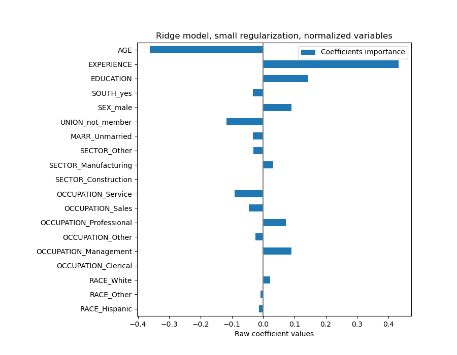
coefs = pd.DataFrame(
    model[-1].regressor_.coef_,
    columns=["Coefficients importance"],
    index=feature_names,
)
coefs.plot.barh(figsize=(9, 7))
plt.title("Ridge model, small regularization, normalized variables")
plt.xlabel("Raw coefficient values")
plt.axvline(x=0, color=".5")
plt.subplots_adjust(left=0.3)
We now inspect the coefficients across several cross-validation folds.
cv_model = cross_validate(
    model,
    X,
    y,
    cv=cv,
    return_estimator=True,
    n_jobs=2,
)
coefs = pd.DataFrame(
    [est[-1].regressor_.coef_ for est in cv_model["estimator"]], columns=feature_names
)
plt.figure(figsize=(9, 7))
sns.stripplot(data=coefs, orient="h", palette="dark:k", alpha=0.5)
sns.boxplot(data=coefs, orient="h", color="cyan", saturation=0.5, whis=10)
plt.axvline(x=0, color=".5")
plt.title("Coefficient variability")
plt.subplots_adjust(left=0.3)
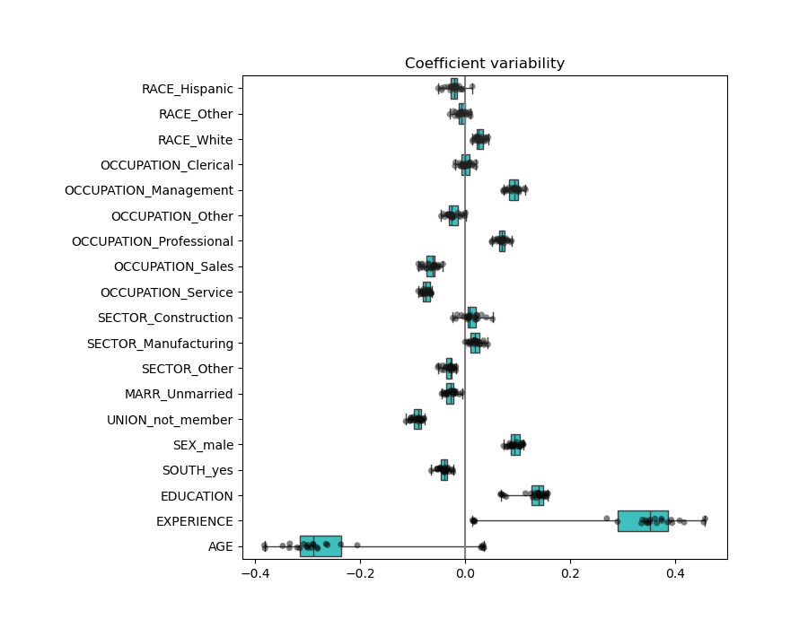
The result is quite similar to the non-normalized case.
Linear models with regularization#
In machine-learning practice, ridge regression is more often used with non-negligible regularization.
Above, we limited this regularization to a very little amount. Regularization
improves the conditioning of the problem and reduces the variance of the
estimates. RidgeCV applies cross validation
in order to determine which value of the regularization parameter (alpha)
is best suited for prediction.
from sklearn.linear_model import RidgeCV

alphas = np.logspace(-10, 10, 21)  # alpha values to be chosen from by cross-validation
model = make_pipeline(
    preprocessor,
    TransformedTargetRegressor(
        regressor=RidgeCV(alphas=alphas),
        func=np.log10,
        inverse_func=sp.special.exp10,
    ),
)
model.fit(X_train, y_train)
First we check which value of \(\alpha\) has been selected.
model[-1].regressor_.alpha_
10.0
Then we check the quality of the predictions.
mae_train = median_absolute_error(y_train, model.predict(X_train))
y_pred = model.predict(X_test)
mae_test = median_absolute_error(y_test, y_pred)
scores = {
    "MedAE on training set": f"{mae_train:.2f} $/hour",
    "MedAE on testing set": f"{mae_test:.2f} $/hour",
}

_, ax = plt.subplots(figsize=(5, 5))
display = PredictionErrorDisplay.from_predictions(
    y_test, y_pred, kind="actual_vs_predicted", ax=ax, scatter_kwargs={"alpha": 0.5}
)
ax.set_title("Ridge model, optimum regularization")
for name, score in scores.items():
    ax.plot([], [], " ", label=f"{name}: {score}")
ax.legend(loc="upper left")
plt.tight_layout()
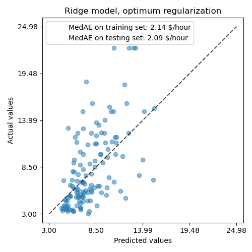
The ability to reproduce the data of the regularized model is similar to the one of the non-regularized model.
coefs = pd.DataFrame(
    model[-1].regressor_.coef_,
    columns=["Coefficients importance"],
    index=feature_names,
)
coefs.plot.barh(figsize=(9, 7))
plt.title("Ridge model, with regularization, normalized variables")
plt.xlabel("Raw coefficient values")
plt.axvline(x=0, color=".5")
plt.subplots_adjust(left=0.3)
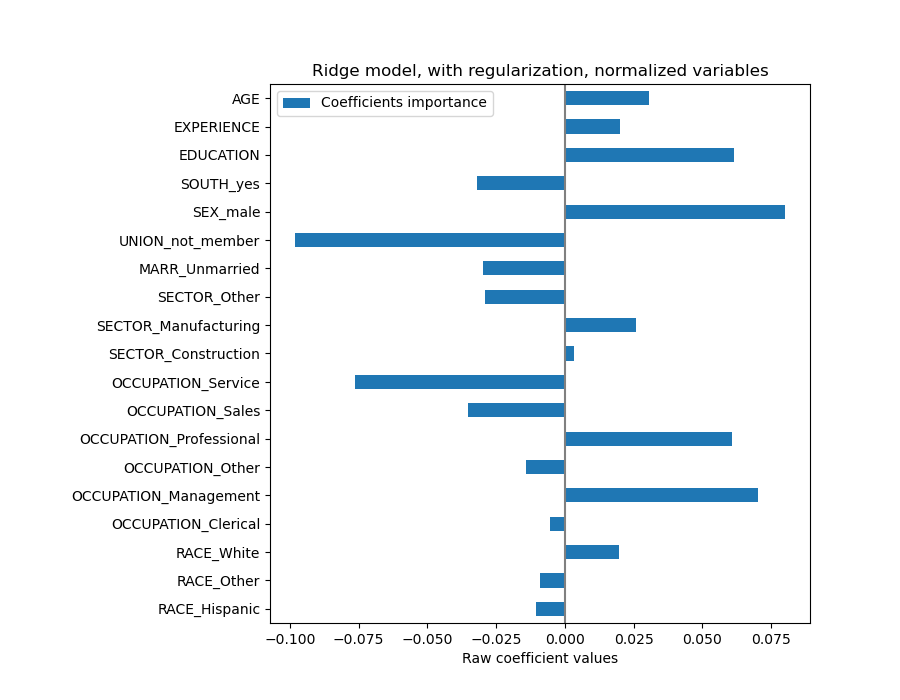
The coefficients are significantly different. AGE and EXPERIENCE coefficients are both positive but they now have less influence on the prediction.
The regularization reduces the influence of correlated variables on the model because the weight is shared between the two predictive variables, so neither alone would have strong weights.
On the other hand, the weights obtained with regularization are more stable (see the Ridge regression and classification User Guide section). This increased stability is visible from the plot, obtained from data perturbations, in a cross-validation. This plot can be compared with the previous one.
cv_model = cross_validate(
    model,
    X,
    y,
    cv=cv,
    return_estimator=True,
    n_jobs=2,
)
coefs = pd.DataFrame(
    [est[-1].regressor_.coef_ for est in cv_model["estimator"]], columns=feature_names
)
plt.xlabel("Age coefficient")
plt.ylabel("Experience coefficient")
plt.grid(True)
plt.xlim(-0.4, 0.5)
plt.ylim(-0.4, 0.5)
plt.scatter(coefs["AGE"], coefs["EXPERIENCE"])
_ = plt.title("Co-variations of coefficients for AGE and EXPERIENCE across folds")
Linear models with sparse coefficients#
Another possibility to take into account correlated variables in the dataset, is to estimate sparse coefficients. In some way we already did it manually when we dropped the AGE column in a previous ridge estimation.
Lasso models (see the Lasso User Guide section) estimates sparse
coefficients. LassoCV applies cross
validation in order to determine which value of the regularization parameter
(alpha) is best suited for the model estimation.
from sklearn.linear_model import LassoCV

alphas = np.logspace(-10, 10, 21)  # alpha values to be chosen from by cross-validation
model = make_pipeline(
    preprocessor,
    TransformedTargetRegressor(
        regressor=LassoCV(alphas=alphas, max_iter=100_000),
        func=np.log10,
        inverse_func=sp.special.exp10,
    ),
)

_ = model.fit(X_train, y_train)
First we verify which value of \(\alpha\) has been selected.
model[-1].regressor_.alpha_
np.float64(0.001)
Then we check the quality of the predictions.
mae_train = median_absolute_error(y_train, model.predict(X_train))
y_pred = model.predict(X_test)
mae_test = median_absolute_error(y_test, y_pred)
scores = {
    "MedAE on training set": f"{mae_train:.2f} $/hour",
    "MedAE on testing set": f"{mae_test:.2f} $/hour",
}

_, ax = plt.subplots(figsize=(6, 6))
display = PredictionErrorDisplay.from_predictions(
    y_test, y_pred, kind="actual_vs_predicted", ax=ax, scatter_kwargs={"alpha": 0.5}
)
ax.set_title("Lasso model, optimum regularization")
for name, score in scores.items():
    ax.plot([], [], " ", label=f"{name}: {score}")
ax.legend(loc="upper left")
plt.tight_layout()
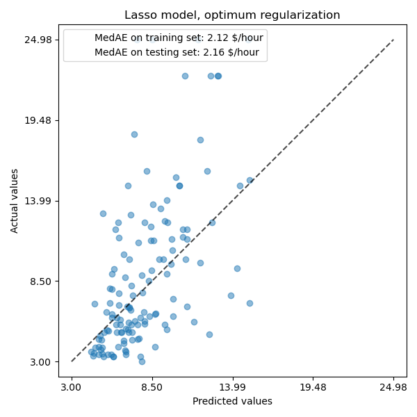
For our dataset, again the model is not very predictive.
coefs = pd.DataFrame(
    model[-1].regressor_.coef_,
    columns=["Coefficients importance"],
    index=feature_names,
)
coefs.plot(kind="barh", figsize=(9, 7))
plt.title("Lasso model, optimum regularization, normalized variables")
plt.axvline(x=0, color=".5")
plt.subplots_adjust(left=0.3)
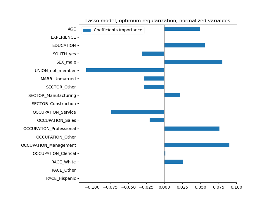
A Lasso model identifies the correlation between AGE and EXPERIENCE and suppresses one of them for the sake of the prediction.
It is important to keep in mind that the coefficients that have been dropped may still be related to the outcome by themselves: the model chose to suppress them because they bring little or no additional information on top of the other features. Additionally, this selection is unstable for correlated features, and should be interpreted with caution.
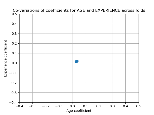
Indeed, we can check the variability of the coefficients across folds.
cv_model = cross_validate(
    model,
    X,
    y,
    cv=cv,
    return_estimator=True,
    n_jobs=2,
)
coefs = pd.DataFrame(
    [est[-1].regressor_.coef_ for est in cv_model["estimator"]], columns=feature_names
)
plt.figure(figsize=(9, 7))
sns.stripplot(data=coefs, orient="h", palette="dark:k", alpha=0.5)
sns.boxplot(data=coefs, orient="h", color="cyan", saturation=0.5, whis=100)
plt.axvline(x=0, color=".5")
plt.title("Coefficient variability")
plt.subplots_adjust(left=0.3)
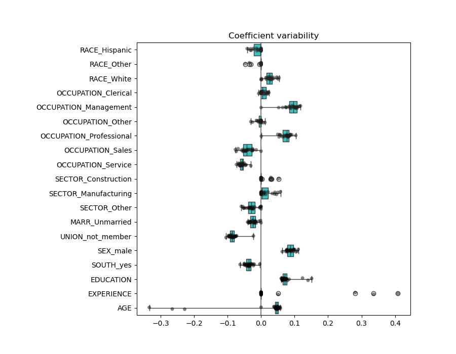
We observe that the AGE and EXPERIENCE coefficients are varying a lot depending of the fold.
Wrong causal interpretation#
Policy makers might want to know the effect of education on wage to assess whether or not a certain policy designed to entice people to pursue more education would make economic sense. While Machine Learning models are great for measuring statistical associations, they are generally unable to infer causal effects.
It might be tempting to look at the coefficient of education on wage from our last model (or any model for that matter) and conclude that it captures the true effect of a change in the standardized education variable on wages.
Unfortunately there are likely unobserved confounding variables that either inflate or deflate that coefficient. A confounding variable is a variable that causes both EDUCATION and WAGE. One example of such variable is ability. Presumably, more able people are more likely to pursue education while at the same time being more likely to earn a higher hourly wage at any level of education. In this case, ability induces a positive Omitted Variable Bias (OVB) on the EDUCATION coefficient, thereby exaggerating the effect of education on wages.
See the Failure of Machine Learning to infer causal effects for a simulated case of ability OVB.
Lessons learned#
Coefficients must be scaled to the same unit of measure to retrieve feature importance. Scaling them with the standard-deviation of the feature is a useful proxy.
Coefficients in multivariate linear models represent the dependency between a given feature and the target, conditional on the other features.
Correlated features induce instabilities in the coefficients of linear models and their effects cannot be well teased apart.
Different linear models respond differently to feature correlation and coefficients could significantly vary from one another.
Inspecting coefficients across the folds of a cross-validation loop gives an idea of their stability.
Interpreting causality is difficult when there are confounding effects. If the relationship between two variables is also affected by something unobserved, we should be careful when making conclusions about causality.
Total running time of the script: (0 minutes 16.545 seconds)
Related examples
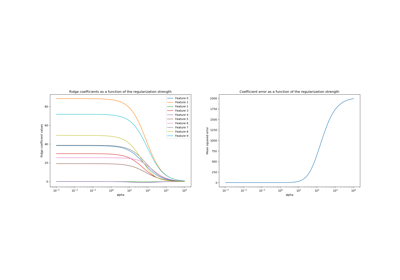
Ridge coefficients as a function of the L2 Regularization
Failure of Machine Learning to infer causal effects
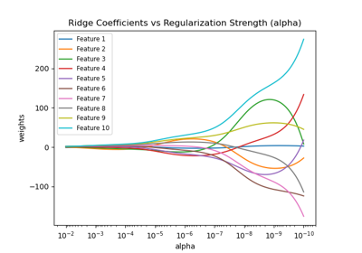
Plot Ridge coefficients as a function of the regularization
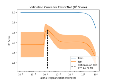
Effect of model regularization on training and test error
