Permutation Importance with Multicollinear or Correlated Features

In this example, we compute the permutation_importance of the features to a trained RandomForestClassifier using the Breast cancer wisconsin (diagnostic) dataset. The model can easily get about 97% accuracy on a test dataset. Because this dataset contains multicollinear features, the permutation importance shows that none of the features are important, in contradiction with the high test accuracy.

We demo a possible approach to handling multicollinearity, which consists of hierarchical clustering on the features’ Spearman rank-order correlations, picking a threshold, and keeping a single feature from each cluster.

Note

See also Permutation Importance vs Random Forest Feature Importance (MDI)

# Authors: The scikit-learn developers
# SPDX-License-Identifier: BSD-3-Clause

Random Forest Feature Importance on Breast Cancer Data

First, we define a function to ease the plotting:

import matplotlib

from sklearn.inspection import permutation_importance
from sklearn.utils.fixes import parse_version


def plot_permutation_importance(clf, X, y, ax):
    result = permutation_importance(clf, X, y, n_repeats=10, random_state=42, n_jobs=2)
    perm_sorted_idx = result.importances_mean.argsort()

    # `labels` argument in boxplot is deprecated in matplotlib 3.9 and has been
    # renamed to `tick_labels`. The following code handles this, but as a
    # scikit-learn user you probably can write simpler code by using `labels=...`
    # (matplotlib < 3.9) or `tick_labels=...` (matplotlib >= 3.9).
    tick_labels_parameter_name = (
        "tick_labels"
        if parse_version(matplotlib.__version__) >= parse_version("3.9")
        else "labels"
    )
    tick_labels_dict = {tick_labels_parameter_name: X.columns[perm_sorted_idx]}
    ax.boxplot(result.importances[perm_sorted_idx].T, vert=False, **tick_labels_dict)
    ax.axvline(x=0, color="k", linestyle="--")
    return ax

We then train a RandomForestClassifier on the Breast cancer wisconsin (diagnostic) dataset and evaluate its accuracy on a test set:

from sklearn.datasets import load_breast_cancer
from sklearn.ensemble import RandomForestClassifier
from sklearn.model_selection import train_test_split

X, y = load_breast_cancer(return_X_y=True, as_frame=True)
X_train, X_test, y_train, y_test = train_test_split(X, y, random_state=42)

clf = RandomForestClassifier(n_estimators=100, random_state=42)
clf.fit(X_train, y_train)
print(f"Baseline accuracy on test data: {clf.score(X_test, y_test):.2}")

Baseline accuracy on test data: 0.97

Next, we plot the tree based feature importance and the permutation importance. The permutation importance is calculated on the training set to show how much the model relies on each feature during training.

import matplotlib.pyplot as plt
import numpy as np
import pandas as pd

mdi_importances = pd.Series(clf.feature_importances_, index=X_train.columns)
tree_importance_sorted_idx = np.argsort(clf.feature_importances_)

fig, (ax1, ax2) = plt.subplots(1, 2, figsize=(12, 8))
mdi_importances.sort_values().plot.barh(ax=ax1)
ax1.set_xlabel("Gini importance")
plot_permutation_importance(clf, X_train, y_train, ax2)
ax2.set_xlabel("Decrease in accuracy score")
fig.suptitle(
    "Impurity-based vs. permutation importances on multicollinear features (train set)"
)
_ = fig.tight_layout()

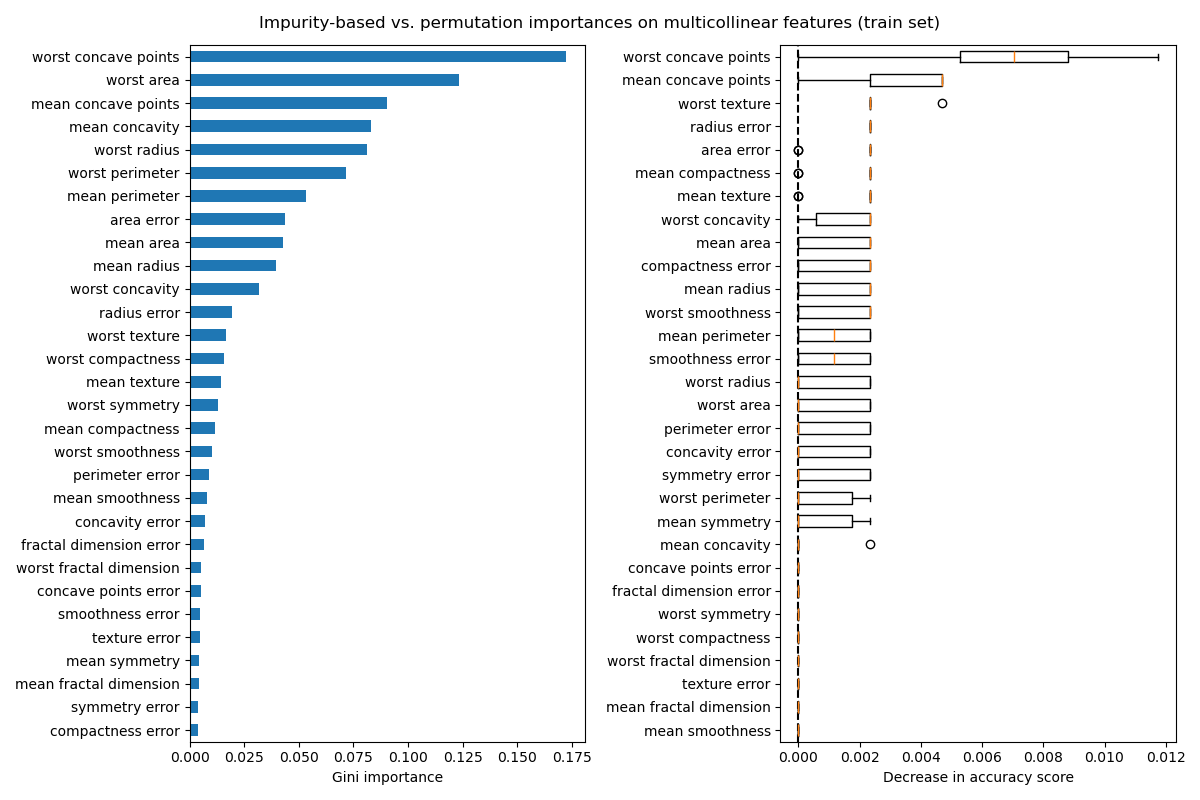
The plot on the left shows the Gini importance of the model. As the scikit-learn implementation of RandomForestClassifier uses a random subsets of \(\sqrt{n_\text{features}}\) features at each split, it is able to dilute the dominance of any single correlated feature. As a result, the individual feature importance may be distributed more evenly among the correlated features. Since the features have large cardinality and the classifier is non-overfitted, we can relatively trust those values.

The permutation importance on the right plot shows that permuting a feature drops the accuracy by at most 0.012, which would suggest that none of the features are important. This is in contradiction with the high test accuracy computed as baseline: some feature must be important.

Similarly, the change in accuracy score computed on the test set appears to be driven by chance:

fig, ax = plt.subplots(figsize=(7, 6))
plot_permutation_importance(clf, X_test, y_test, ax)
ax.set_title("Permutation Importances on multicollinear features\n(test set)")
ax.set_xlabel("Decrease in accuracy score")
_ = ax.figure.tight_layout()

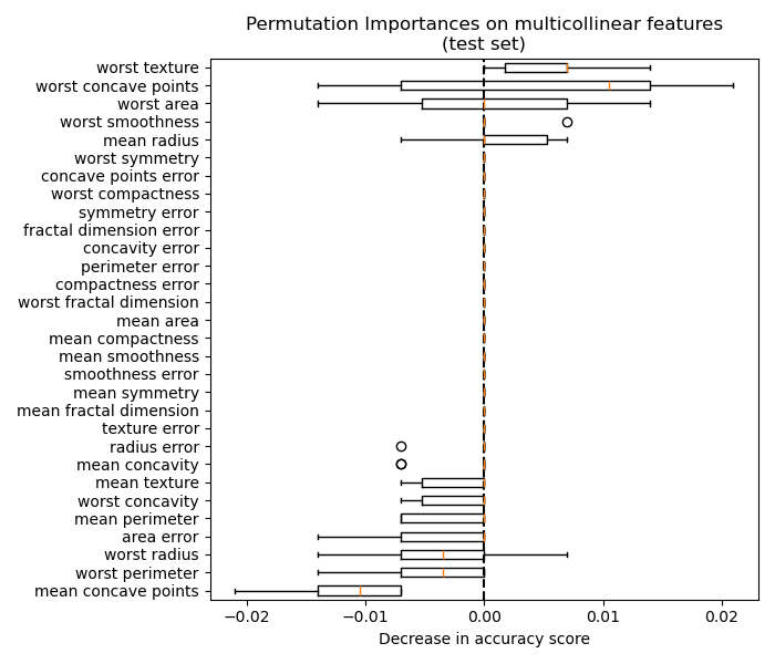
Nevertheless, one can still compute a meaningful permutation importance in the presence of correlated features, as demonstrated in the following section.

Handling Multicollinear Features

When features are collinear, permuting one feature has little effect on the models performance because it can get the same information from a correlated feature. Note that this is not the case for all predictive models and depends on their underlying implementation.

One way to handle multicollinear features is by performing hierarchical clustering on the Spearman rank-order correlations, picking a threshold, and keeping a single feature from each cluster. First, we plot a heatmap of the correlated features:

from scipy.cluster import hierarchy
from scipy.spatial.distance import squareform
from scipy.stats import spearmanr

fig, (ax1, ax2) = plt.subplots(1, 2, figsize=(12, 8))
corr = spearmanr(X).correlation

# Ensure the correlation matrix is symmetric
corr = (corr + corr.T) / 2
np.fill_diagonal(corr, 1)

# We convert the correlation matrix to a distance matrix before performing
# hierarchical clustering using Ward's linkage.
distance_matrix = 1 - np.abs(corr)
dist_linkage = hierarchy.ward(squareform(distance_matrix))
dendro = hierarchy.dendrogram(
    dist_linkage, labels=X.columns.to_list(), ax=ax1, leaf_rotation=90
)
dendro_idx = np.arange(0, len(dendro["ivl"]))

ax2.imshow(corr[dendro["leaves"], :][:, dendro["leaves"]])
ax2.set_xticks(dendro_idx)
ax2.set_yticks(dendro_idx)
ax2.set_xticklabels(dendro["ivl"], rotation="vertical")
ax2.set_yticklabels(dendro["ivl"])
_ = fig.tight_layout()

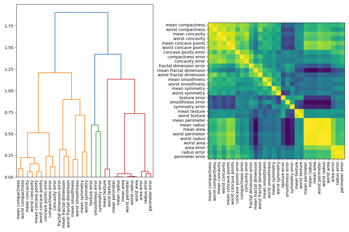
Next, we manually pick a threshold by visual inspection of the dendrogram to group our features into clusters and choose a feature from each cluster to keep, select those features from our dataset, and train a new random forest. The test accuracy of the new random forest did not change much compared to the random forest trained on the complete dataset.

from collections import defaultdict

cluster_ids = hierarchy.fcluster(dist_linkage, 1, criterion="distance")
cluster_id_to_feature_ids = defaultdict(list)
for idx, cluster_id in enumerate(cluster_ids):
    cluster_id_to_feature_ids[cluster_id].append(idx)
selected_features = [v[0] for v in cluster_id_to_feature_ids.values()]
selected_features_names = X.columns[selected_features]

X_train_sel = X_train[selected_features_names]
X_test_sel = X_test[selected_features_names]

clf_sel = RandomForestClassifier(n_estimators=100, random_state=42)
clf_sel.fit(X_train_sel, y_train)
print(
    "Baseline accuracy on test data with features removed:"
    f" {clf_sel.score(X_test_sel, y_test):.2}"
)

Baseline accuracy on test data with features removed: 0.97

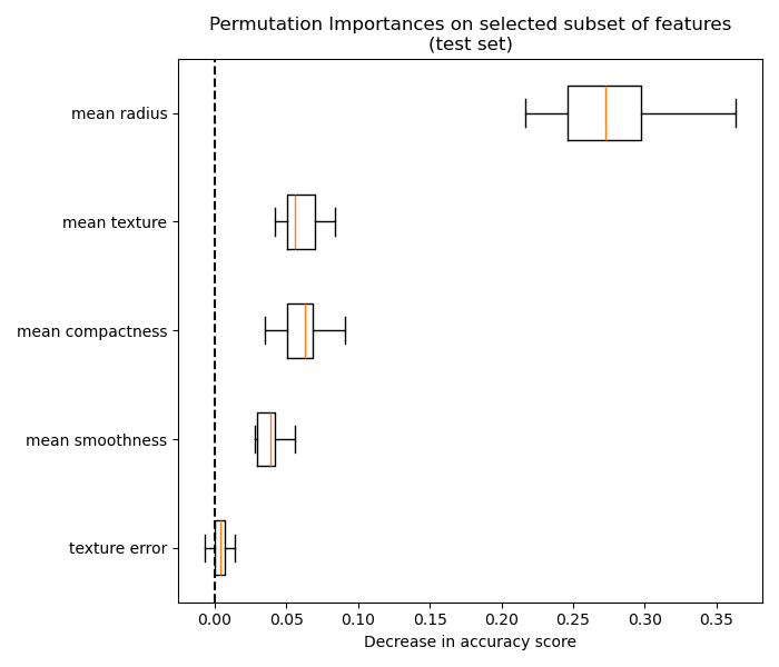
We can finally explore the permutation importance of the selected subset of features:

fig, ax = plt.subplots(figsize=(7, 6))
plot_permutation_importance(clf_sel, X_test_sel, y_test, ax)
ax.set_title("Permutation Importances on selected subset of features\n(test set)")
ax.set_xlabel("Decrease in accuracy score")
ax.figure.tight_layout()
plt.show()

Related examples

Permutation Importance vs Random Forest Feature Importance (MDI)

Permutation Importance vs Random Forest Feature Importance (MDI)

Feature importances with a forest of trees

Feature importances with a forest of trees

Gradient Boosting regression

Gradient Boosting regression

Effect of varying threshold for self-training

Effect of varying threshold for self-training