2.6. Covariance estimation#
Many statistical problems require the estimation of a
population’s covariance matrix, which can be seen as an estimation of
data set scatter plot shape. Most of the time, such an estimation has
to be done on a sample whose properties (size, structure, homogeneity)
have a large influence on the estimation’s quality. The
sklearn.covariance package provides tools for accurately estimating
a population’s covariance matrix under various settings.
We assume that the observations are independent and identically distributed (i.i.d.).
2.6.1. Empirical covariance#
The covariance matrix of a data set is known to be well approximated by the classical maximum likelihood estimator (or “empirical covariance”), provided the number of observations is large enough compared to the number of features (the variables describing the observations). More precisely, the Maximum Likelihood Estimator of a sample is an asymptotically unbiased estimator of the corresponding population’s covariance matrix.
The empirical covariance matrix of a sample can be computed using the
empirical_covariance function of the package, or by fitting an
EmpiricalCovariance object to the data sample with the
EmpiricalCovariance.fit method. Be careful that results depend
on whether the data are centered, so one may want to use the
assume_centered parameter accurately. More precisely, if assume_centered=True, then
all features in the train and test sets should have a mean of zero. If not, both should
be centered by the user, or assume_centered=False should be used.
Examples
See Shrinkage covariance estimation: LedoitWolf vs OAS and max-likelihood for an example on how to fit an
EmpiricalCovarianceobject to data.
2.6.2. Shrunk Covariance#
2.6.2.1. Basic shrinkage#
Despite being an asymptotically unbiased estimator of the covariance matrix,
the Maximum Likelihood Estimator is not a good estimator of the
eigenvalues of the covariance matrix, so the precision matrix obtained
from its inversion is not accurate. Sometimes, it even occurs that the
empirical covariance matrix cannot be inverted for numerical
reasons. To avoid such an inversion problem, a transformation of the
empirical covariance matrix has been introduced: the shrinkage.
In scikit-learn, this transformation (with a user-defined shrinkage
coefficient) can be directly applied to a pre-computed covariance with
the shrunk_covariance method. Also, a shrunk estimator of the
covariance can be fitted to data with a ShrunkCovariance object
and its ShrunkCovariance.fit method. Again, results depend on
whether the data are centered, so one may want to use the
assume_centered parameter accurately.
Mathematically, this shrinkage consists in reducing the ratio between the smallest and the largest eigenvalues of the empirical covariance matrix. It can be done by simply shifting every eigenvalue according to a given offset, which is equivalent of finding the l2-penalized Maximum Likelihood Estimator of the covariance matrix. In practice, shrinkage boils down to a simple convex transformation : \(\Sigma_{\rm shrunk} = (1-\alpha)\hat{\Sigma} + \alpha\frac{{\rm Tr}\hat{\Sigma}}{p}\rm Id\).
Choosing the amount of shrinkage, \(\alpha\) amounts to setting a bias/variance trade-off, and is discussed below.
Examples
See Shrinkage covariance estimation: LedoitWolf vs OAS and max-likelihood for an example on how to fit a
ShrunkCovarianceobject to data.
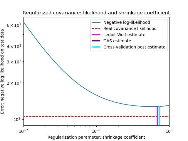
2.6.2.2. Ledoit-Wolf shrinkage#
In their 2004 paper [1], O. Ledoit and M. Wolf propose a formula to compute the optimal shrinkage coefficient \(\alpha\) that minimizes the Mean Squared Error between the estimated and the real covariance matrix.
The Ledoit-Wolf estimator of the covariance matrix can be computed on
a sample with the ledoit_wolf function of the
sklearn.covariance package, or it can be otherwise obtained by
fitting a LedoitWolf object to the same sample.
Note
Case when population covariance matrix is isotropic
It is important to note that when the number of samples is much larger than the number of features, one would expect that no shrinkage would be necessary. The intuition behind this is that if the population covariance is full rank, when the number of samples grows, the sample covariance will also become positive definite. As a result, no shrinkage would be necessary and the method should automatically do this.
This, however, is not the case in the Ledoit-Wolf procedure when the population covariance happens to be a multiple of the identity matrix. In this case, the Ledoit-Wolf shrinkage estimate approaches 1 as the number of samples increases. This indicates that the optimal estimate of the covariance matrix in the Ledoit-Wolf sense is a multiple of the identity. Since the population covariance is already a multiple of the identity matrix, the Ledoit-Wolf solution is indeed a reasonable estimate.
Examples
See Shrinkage covariance estimation: LedoitWolf vs OAS and max-likelihood for an example on how to fit a
LedoitWolfobject to data and for visualizing the performances of the Ledoit-Wolf estimator in terms of likelihood.
References
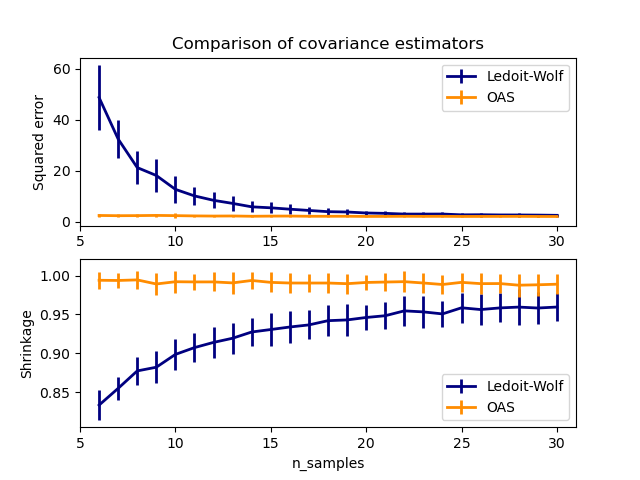
2.6.2.3. Oracle Approximating Shrinkage#
Under the assumption that the data are Gaussian distributed, Chen et al. [2] derived a formula aimed at choosing a shrinkage coefficient that yields a smaller Mean Squared Error than the one given by Ledoit and Wolf’s formula. The resulting estimator is known as the Oracle Shrinkage Approximating estimator of the covariance.
The OAS estimator of the covariance matrix can be computed on a sample
with the oas function of the sklearn.covariance
package, or it can be otherwise obtained by fitting an OAS
object to the same sample.
Bias-variance trade-off when setting the shrinkage: comparing the choices of Ledoit-Wolf and OAS estimators#
References
Examples
See Shrinkage covariance estimation: LedoitWolf vs OAS and max-likelihood for an example on how to fit an
OASobject to data.See Ledoit-Wolf vs OAS estimation to visualize the Mean Squared Error difference between a
LedoitWolfand anOASestimator of the covariance.
2.6.3. Sparse inverse covariance#
The matrix inverse of the covariance matrix, often called the precision matrix, is proportional to the partial correlation matrix. It gives the partial independence relationship. In other words, if two features are independent conditionally on the others, the corresponding coefficient in the precision matrix will be zero. This is why it makes sense to estimate a sparse precision matrix: the estimation of the covariance matrix is better conditioned by learning independence relations from the data. This is known as covariance selection.
In the small-samples situation, in which n_samples is on the order
of n_features or smaller, sparse inverse covariance estimators tend to work
better than shrunk covariance estimators. However, in the opposite
situation, or for very correlated data, they can be numerically unstable.
In addition, unlike shrinkage estimators, sparse estimators are able to
recover off-diagonal structure.
The GraphicalLasso estimator uses an l1 penalty to enforce sparsity on
the precision matrix: the higher its alpha parameter, the more sparse
the precision matrix. The corresponding GraphicalLassoCV object uses
cross-validation to automatically set the alpha parameter.
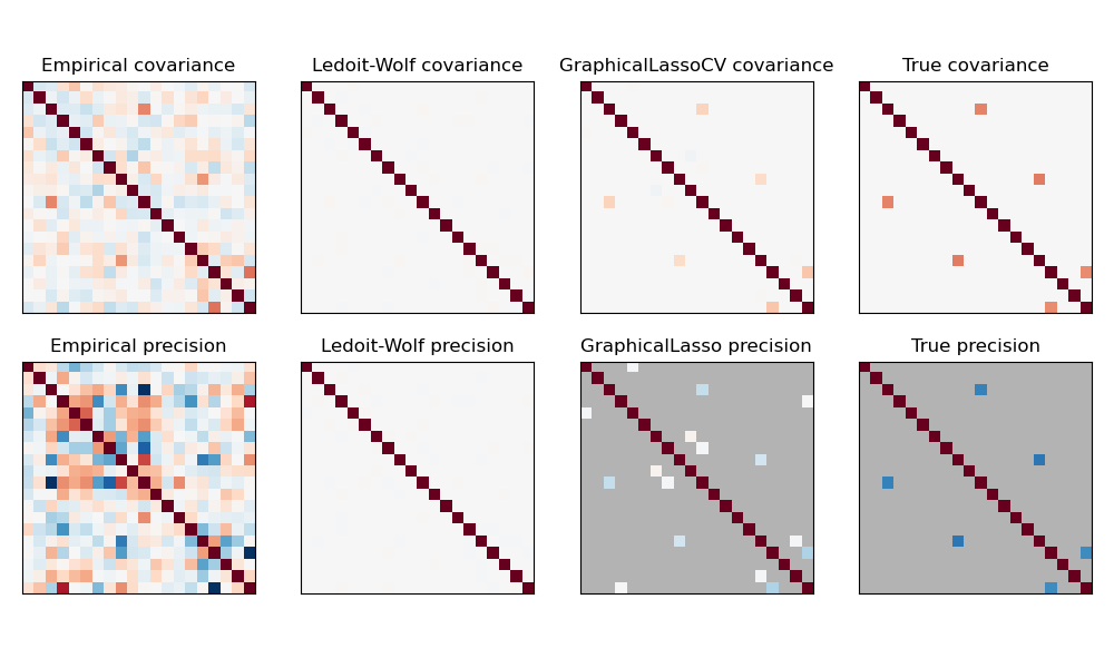
A comparison of maximum likelihood, shrinkage and sparse estimates of the covariance and precision matrix in the very small samples settings.#
Note
Structure recovery
Recovering a graphical structure from correlations in the data is a challenging thing. If you are interested in such recovery keep in mind that:
Recovery is easier from a correlation matrix than a covariance matrix: standardize your observations before running
GraphicalLassoIf the underlying graph has nodes with much more connections than the average node, the algorithm will miss some of these connections.
If your number of observations is not large compared to the number of edges in your underlying graph, you will not recover it.
Even if you are in favorable recovery conditions, the alpha parameter chosen by cross-validation (e.g. using the
GraphicalLassoCVobject) will lead to selecting too many edges. However, the relevant edges will have heavier weights than the irrelevant ones.
The mathematical formulation is the following:
Where \(K\) is the precision matrix to be estimated, and \(S\) is the
sample covariance matrix. \(\|K\|_1\) is the sum of the absolute values of
off-diagonal coefficients of \(K\). The algorithm employed to solve this
problem is the GLasso algorithm, from the Friedman 2008 Biostatistics
paper. It is the same algorithm as in the R glasso package.
Examples
Sparse inverse covariance estimation: example on synthetic data showing some recovery of a structure, and comparing to other covariance estimators.
Visualizing the stock market structure: example on real stock market data, finding which symbols are most linked.
References
Friedman et al, “Sparse inverse covariance estimation with the graphical lasso”, Biostatistics 9, pp 432, 2008
2.6.4. Robust Covariance Estimation#
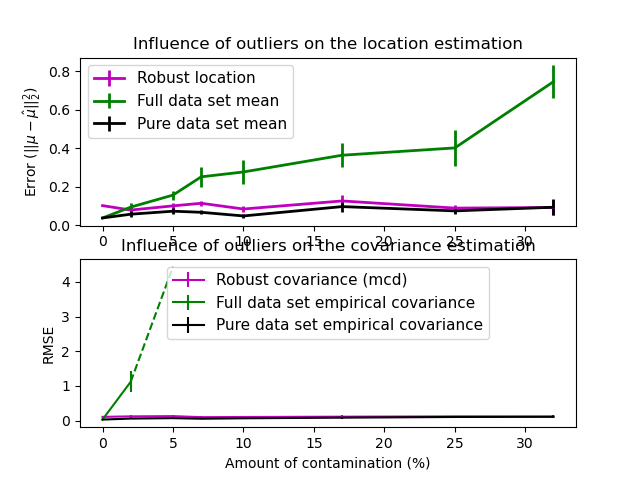
Real data sets are often subject to measurement or recording errors. Regular but uncommon observations may also appear for a variety of reasons. Observations which are very uncommon are called outliers. The empirical covariance estimator and the shrunk covariance estimators presented above are very sensitive to the presence of outliers in the data. Therefore, one should use robust covariance estimators to estimate the covariance of its real data sets. Alternatively, robust covariance estimators can be used to perform outlier detection and discard/downweight some observations according to further processing of the data.
The sklearn.covariance package implements a robust estimator of covariance,
the Minimum Covariance Determinant [3].
2.6.4.1. Minimum Covariance Determinant#
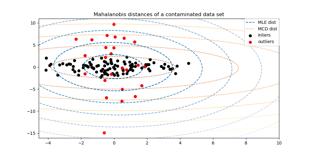
The Minimum Covariance Determinant estimator is a robust estimator of a data set’s covariance introduced by P.J. Rousseeuw in [3]. The idea is to find a given proportion (h) of “good” observations which are not outliers and compute their empirical covariance matrix. This empirical covariance matrix is then rescaled to compensate the performed selection of observations (“consistency step”). Having computed the Minimum Covariance Determinant estimator, one can give weights to observations according to their Mahalanobis distance, leading to a reweighted estimate of the covariance matrix of the data set (“reweighting step”).
Rousseeuw and Van Driessen [4] developed the FastMCD algorithm in order to compute the Minimum Covariance Determinant. This algorithm is used in scikit-learn when fitting an MCD object to data. The FastMCD algorithm also computes a robust estimate of the data set location at the same time.
Raw estimates can be accessed as raw_location_ and raw_covariance_
attributes of a MinCovDet robust covariance estimator object.
References
Examples
See Robust vs Empirical covariance estimate for an example on how to fit a
MinCovDetobject to data and see how the estimate remains accurate despite the presence of outliers.See Robust covariance estimation and Mahalanobis distances relevance to visualize the difference between
EmpiricalCovarianceandMinCovDetcovariance estimators in terms of Mahalanobis distance (so we get a better estimate of the precision matrix too).
Influence of outliers on location and covariance estimates |
Separating inliers from outliers using a Mahalanobis distance |
|---|---|
|
|