1.11. Ensembles: Gradient boosting, random forests, bagging, voting, stacking#
Ensemble methods combine the predictions of several base estimators built with a given learning algorithm in order to improve generalizability / robustness over a single estimator.
Two very famous examples of ensemble methods are gradient-boosted trees and random forests.
More generally, ensemble models can be applied to any base learner beyond trees, in averaging methods such as Bagging methods, model stacking, or Voting, or in boosting, as AdaBoost.
1.11.1. Gradient-boosted trees#
Gradient Tree Boosting or Gradient Boosted Decision Trees (GBDT) is a generalization of boosting to arbitrary differentiable loss functions, see the seminal work of [Friedman2001]. GBDT is an excellent model for both regression and classification, in particular for tabular data.
1.11.1.1. Histogram-Based Gradient Boosting#
Scikit-learn 0.21 introduced two new implementations of
gradient boosted trees, namely HistGradientBoostingClassifier
and HistGradientBoostingRegressor, inspired by
LightGBM (See [LightGBM]).
These histogram-based estimators can be orders of magnitude faster
than GradientBoostingClassifier and
GradientBoostingRegressor when the number of samples is larger
than tens of thousands of samples.
They also have built-in support for missing values, which avoids the need for an imputer.
These fast estimators first bin the input samples X into
integer-valued bins (typically 256 bins) which tremendously reduces the
number of splitting points to consider, and allows the algorithm to
leverage integer-based data structures (histograms) instead of relying on
sorted continuous values when building the trees. The API of these
estimators is slightly different, and some of the features from
GradientBoostingClassifier and GradientBoostingRegressor
are not yet supported, for instance some loss functions.
Examples
Partial Dependence and Individual Conditional Expectation Plots
Comparing Random Forests and Histogram Gradient Boosting models
1.11.1.1.1. Usage#
Most of the parameters are unchanged from
GradientBoostingClassifier and GradientBoostingRegressor.
One exception is the max_iter parameter that replaces n_estimators, and
controls the number of iterations of the boosting process:
>>> from sklearn.ensemble import HistGradientBoostingClassifier
>>> from sklearn.datasets import make_hastie_10_2

>>> X, y = make_hastie_10_2(random_state=0)
>>> X_train, X_test = X[:2000], X[2000:]
>>> y_train, y_test = y[:2000], y[2000:]

>>> clf = HistGradientBoostingClassifier(max_iter=100).fit(X_train, y_train)
>>> clf.score(X_test, y_test)
0.8965
Available losses for regression are:
‘squared_error’, which is the default loss;
‘absolute_error’, which is less sensitive to outliers than the squared error;
‘gamma’, which is well suited to model strictly positive outcomes;
‘poisson’, which is well suited to model counts and frequencies;
‘quantile’, which allows for estimating a conditional quantile that can later be used to obtain prediction intervals.
For classification, ‘log_loss’ is the only option. For binary classification
it uses the binary log loss, also known as binomial deviance or binary
cross-entropy. For n_classes >= 3, it uses the multi-class log loss function,
with multinomial deviance and categorical cross-entropy as alternative names.
The appropriate loss version is selected based on y passed to
fit.
The size of the trees can be controlled through the max_leaf_nodes,
max_depth, and min_samples_leaf parameters.
The number of bins used to bin the data is controlled with the max_bins
parameter. Using less bins acts as a form of regularization. It is generally
recommended to use as many bins as possible (255), which is the default.
The l2_regularization parameter acts as a regularizer for the loss function,
and corresponds to \(\lambda\) in the following expression (see equation (2)
in [XGBoost]):
Details on l2 regularization#
It is important to notice that the loss term \(l(\hat{y}_i, y_i)\) describes only half of the actual loss function except for the pinball loss and absolute error.
The index \(k\) refers to the k-th tree in the ensemble of trees. In the
case of regression and binary classification, gradient boosting models grow one
tree per iteration, then \(k\) runs up to max_iter. In the case of
multiclass classification problems, the maximal value of the index \(k\) is
n_classes \(\times\) max_iter.
If \(T_k\) denotes the number of leaves in the k-th tree, then \(w_k\)
is a vector of length \(T_k\), which contains the leaf values of the form w
= -sum_gradient / (sum_hessian + l2_regularization) (see equation (5) in
[XGBoost]).
The leaf values \(w_k\) are derived by dividing the sum of the gradients of the loss function by the combined sum of hessians. Adding the regularization to the denominator penalizes the leaves with small hessians (flat regions), resulting in smaller updates. Those \(w_k\) values contribute then to the model’s prediction for a given input that ends up in the corresponding leaf. The final prediction is the sum of the base prediction and the contributions from each tree. The result of that sum is then transformed by the inverse link function depending on the choice of the loss function (see Mathematical formulation).
Notice that the original paper [XGBoost] introduces a term \(\gamma\sum_k
T_k\) that penalizes the number of leaves (making it a smooth version of
max_leaf_nodes) not presented here as it is not implemented in scikit-learn;
whereas \(\lambda\) penalizes the magnitude of the individual tree
predictions before being rescaled by the learning rate, see
Shrinkage via learning rate.
Note that early-stopping is enabled by default if the number of samples is
larger than 10,000. The early-stopping behaviour is controlled via the
early_stopping, scoring, validation_fraction,
n_iter_no_change, and tol parameters. It is possible to early-stop
using an arbitrary scorer, or just the training or validation loss.
Note that for technical reasons, using a callable as a scorer is significantly slower
than using the loss. By default, early-stopping is performed if there are at least
10,000 samples in the training set, using the validation loss.
1.11.1.1.2. Missing values support#
HistGradientBoostingClassifier and
HistGradientBoostingRegressor have built-in support for missing
values (NaNs).
During training, the tree grower learns at each split point whether samples with missing values should go to the left or right child, based on the potential gain. When predicting, samples with missing values are assigned to the left or right child consequently:
>>> from sklearn.ensemble import HistGradientBoostingClassifier
>>> import numpy as np

>>> X = np.array([0, 1, 2, np.nan]).reshape(-1, 1)
>>> y = [0, 0, 1, 1]

>>> gbdt = HistGradientBoostingClassifier(min_samples_leaf=1).fit(X, y)
>>> gbdt.predict(X)
array([0, 0, 1, 1])
When the missingness pattern is predictive, the splits can be performed on whether the feature value is missing or not:
>>> X = np.array([0, np.nan, 1, 2, np.nan]).reshape(-1, 1)
>>> y = [0, 1, 0, 0, 1]
>>> gbdt = HistGradientBoostingClassifier(min_samples_leaf=1,
...                                       max_depth=2,
...                                       learning_rate=1,
...                                       max_iter=1).fit(X, y)
>>> gbdt.predict(X)
array([0, 1, 0, 0, 1])
If no missing values were encountered for a given feature during training, then samples with missing values are mapped to whichever child has the most samples.
Examples
1.11.1.1.3. Sample weight support#
HistGradientBoostingClassifier and
HistGradientBoostingRegressor support sample weights during
fit.
The following toy example demonstrates that samples with a sample weight of zero are ignored:
>>> X = [[1, 0],
...      [1, 0],
...      [1, 0],
...      [0, 1]]
>>> y = [0, 0, 1, 0]
>>> # ignore the first 2 training samples by setting their weight to 0
>>> sample_weight = [0, 0, 1, 1]
>>> gb = HistGradientBoostingClassifier(min_samples_leaf=1)
>>> gb.fit(X, y, sample_weight=sample_weight)
HistGradientBoostingClassifier(...)
>>> gb.predict([[1, 0]])
array([1])
>>> gb.predict_proba([[1, 0]])[0, 1]
np.float64(0.999)
As you can see, the [1, 0] is comfortably classified as 1 since the first
two samples are ignored due to their sample weights.
Implementation detail: taking sample weights into account amounts to multiplying the gradients (and the hessians) by the sample weights. Note that the binning stage (specifically the quantiles computation) does not take the weights into account.
1.11.1.1.4. Categorical Features Support#
HistGradientBoostingClassifier and
HistGradientBoostingRegressor have native support for categorical
features: they can consider splits on non-ordered, categorical data.
For datasets with categorical features, using the native categorical support
is often better than relying on one-hot encoding
(OneHotEncoder), because one-hot encoding
requires more tree depth to achieve equivalent splits. It is also usually
better to rely on the native categorical support rather than to treat
categorical features as continuous (ordinal), which happens for ordinal-encoded
categorical data, since categories are nominal quantities where order does not
matter.
To enable categorical support, a boolean mask can be passed to the
categorical_features parameter, indicating which feature is categorical. In
the following, the first feature will be treated as categorical and the
second feature as numerical:
>>> gbdt = HistGradientBoostingClassifier(categorical_features=[True, False])
Equivalently, one can pass a list of integers indicating the indices of the categorical features:
>>> gbdt = HistGradientBoostingClassifier(categorical_features=[0])
When the input is a DataFrame, it is also possible to pass a list of column names:
>>> gbdt = HistGradientBoostingClassifier(categorical_features=["site", "manufacturer"])
Finally, when the input is a DataFrame we can use
categorical_features="from_dtype" in which case all columns with a categorical
dtype will be treated as categorical features.
The cardinality of each categorical feature must be less than the max_bins
parameter. For an example using histogram-based gradient boosting on categorical
features, see
Categorical Feature Support in Gradient Boosting.
If there are missing values during training, the missing values will be treated as a proper category. If there are no missing values during training, then at prediction time, missing values are mapped to the child node that has the most samples (just like for continuous features). When predicting, categories that were not seen during fit time will be treated as missing values.
Split finding with categorical features#
The canonical way of considering categorical splits in a tree is to consider
all of the \(2^{K - 1} - 1\) partitions, where \(K\) is the number of
categories. This can quickly become prohibitive when \(K\) is large.
Fortunately, since gradient boosting trees are always regression trees (even
for classification problems), there exists a faster strategy that can yield
equivalent splits. First, the categories of a feature are sorted according to
the variance of the target, for each category k. Once the categories are
sorted, one can consider continuous partitions, i.e. treat the categories
as if they were ordered continuous values (see Fisher [Fisher1958] for a
formal proof). As a result, only \(K - 1\) splits need to be considered
instead of \(2^{K - 1} - 1\). The initial sorting is a
\(\mathcal{O}(K \log(K))\) operation, leading to a total complexity of
\(\mathcal{O}(K \log(K) + K)\), instead of \(\mathcal{O}(2^K)\).
Examples
1.11.1.1.5. Monotonic Constraints#
Depending on the problem at hand, you may have prior knowledge indicating that a given feature should in general have a positive (or negative) effect on the target value. For example, all else being equal, a higher credit score should increase the probability of getting approved for a loan. Monotonic constraints allow you to incorporate such prior knowledge into the model.
For a predictor \(F\) with two features:
a monotonic increase constraint is a constraint of the form:
\[x_1 \leq x_1' \implies F(x_1, x_2) \leq F(x_1', x_2)\]a monotonic decrease constraint is a constraint of the form:
\[x_1 \leq x_1' \implies F(x_1, x_2) \geq F(x_1', x_2)\]
You can specify a monotonic constraint on each feature using the
monotonic_cst parameter. For each feature, a value of 0 indicates no
constraint, while 1 and -1 indicate a monotonic increase and
monotonic decrease constraint, respectively:
>>> from sklearn.ensemble import HistGradientBoostingRegressor

... # monotonic increase, monotonic decrease, and no constraint on the 3 features
>>> gbdt = HistGradientBoostingRegressor(monotonic_cst=[1, -1, 0])
In a binary classification context, imposing a monotonic increase (decrease) constraint means that higher values of the feature are supposed to have a positive (negative) effect on the probability of samples to belong to the positive class.
Nevertheless, monotonic constraints only marginally constrain feature effects on the output. For instance, monotonic increase and decrease constraints cannot be used to enforce the following modelling constraint:
Also, monotonic constraints are not supported for multiclass classification.
For a practical implementation of monotonic constraints with the histogram-based gradient boosting, including how they can improve generalization when domain knowledge is available, see Monotonic Constraints.
Note
Since categories are unordered quantities, it is not possible to enforce monotonic constraints on categorical features.
Examples
1.11.1.1.6. Interaction constraints#
A priori, the histogram gradient boosted trees are allowed to use any feature
to split a node into child nodes. This creates so called interactions between
features, i.e. usage of different features as split along a branch. Sometimes,
one wants to restrict the possible interactions, see [Mayer2022]. This can be
done by the parameter interaction_cst, where one can specify the indices
of features that are allowed to interact.
For instance, with 3 features in total, interaction_cst=[{0}, {1}, {2}]
forbids all interactions.
The constraints [{0, 1}, {1, 2}] specify two groups of possibly
interacting features. Features 0 and 1 may interact with each other, as well
as features 1 and 2. But note that features 0 and 2 are forbidden to interact.
The following depicts a tree and the possible splits of the tree:
   1      <- Both constraint groups could be applied from now on
  / \
 1   2    <- Left split still fulfills both constraint groups.
/ \ / \      Right split at feature 2 has only group {1, 2} from now on.
LightGBM uses the same logic for overlapping groups.
Note that features not listed in interaction_cst are automatically
assigned an interaction group for themselves. With again 3 features, this
means that [{0}] is equivalent to [{0}, {1, 2}].
Examples
References
M. Mayer, S.C. Bourassa, M. Hoesli, and D.F. Scognamiglio. 2022. Machine Learning Applications to Land and Structure Valuation. Journal of Risk and Financial Management 15, no. 5: 193
1.11.1.1.7. Low-level parallelism#
HistGradientBoostingClassifier and
HistGradientBoostingRegressor use OpenMP
for parallelization through Cython. For more details on how to control the
number of threads, please refer to our Parallelism notes.
The following parts are parallelized:
mapping samples from real values to integer-valued bins (finding the bin thresholds is however sequential)
building histograms is parallelized over features
finding the best split point at a node is parallelized over features
during fit, mapping samples into the left and right children is parallelized over samples
gradient and hessians computations are parallelized over samples
predicting is parallelized over samples
1.11.1.1.8. Why it’s faster#
The bottleneck of a gradient boosting procedure is building the decision
trees. Building a traditional decision tree (as in the other GBDTs
GradientBoostingClassifier and GradientBoostingRegressor)
requires sorting the samples at each node (for
each feature). Sorting is needed so that the potential gain of a split point
can be computed efficiently. Splitting a single node has thus a complexity
of \(\mathcal{O}(n_\text{features} \times n \log(n))\) where \(n\)
is the number of samples at the node.
HistGradientBoostingClassifier and
HistGradientBoostingRegressor, in contrast, do not require sorting the
feature values and instead use a data-structure called
histogram , where the
samples are implicitly ordered. Building a histogram has a
\(\mathcal{O}(n)\) complexity, so the node splitting procedure has a
\(\mathcal{O}(n_\text{features} \times n)\) complexity, much smaller
than the previous one. In addition, instead of considering \(n\) split
points, we consider only max_bins split points, which might be much
smaller.
In order to build histograms, the input data X needs to be binned into
integer-valued bins. This binning procedure does require sorting the feature
values, but it only happens once at the very beginning of the boosting process
(not at each node, like in GradientBoostingClassifier and
GradientBoostingRegressor).
A second major reason for being faster is the fact that
HistGradientBoostingClassifier and HistGradientBoostingRegressor both
use second order information about the loss, i.e. the Hessian. This is called Newton
boosting and avoids the line-search step of the ordinary gradient boosting.
Finally, many parts of the implementation of
HistGradientBoostingClassifier and
HistGradientBoostingRegressor are parallelized.
References
Fisher, W.D. (1958). “On Grouping for Maximum Homogeneity” Journal of the American Statistical Association, 53, 789-798.
1.11.1.2. GradientBoostingClassifier and GradientBoostingRegressor#
The usage and the parameters of GradientBoostingClassifier and
GradientBoostingRegressor are described below. The 2 most important
parameters of these estimators are n_estimators and learning_rate.
Classification#
GradientBoostingClassifier supports both binary and multi-class
classification.
The following example shows how to fit a gradient boosting classifier
with 100 decision stumps as weak learners:
>>> from sklearn.datasets import make_hastie_10_2
>>> from sklearn.ensemble import GradientBoostingClassifier

>>> X, y = make_hastie_10_2(random_state=0)
>>> X_train, X_test = X[:2000], X[2000:]
>>> y_train, y_test = y[:2000], y[2000:]

>>> clf = GradientBoostingClassifier(n_estimators=100, learning_rate=1.0,
...     max_depth=1, random_state=0).fit(X_train, y_train)
>>> clf.score(X_test, y_test)
0.913
The number of weak learners (i.e. regression trees) is controlled by the
parameter n_estimators; The size of each tree can be controlled either by setting the tree
depth via max_depth or by setting the number of leaf nodes via
max_leaf_nodes. The learning_rate is a hyper-parameter in the range
(0.0, 1.0] that controls overfitting via shrinkage .
Note
Classification with more than 2 classes requires the induction
of n_classes regression trees at each iteration,
thus, the total number of induced trees equals
n_classes * n_estimators. For datasets with a large number
of classes we strongly recommend to use
HistGradientBoostingClassifier as an alternative to
GradientBoostingClassifier .
Regression#
GradientBoostingRegressor supports a number of
different loss functions
for regression which can be specified via the argument
loss; the default loss function for regression is squared error
('squared_error').
>>> import numpy as np
>>> from sklearn.metrics import mean_squared_error
>>> from sklearn.datasets import make_friedman1
>>> from sklearn.ensemble import GradientBoostingRegressor

>>> X, y = make_friedman1(n_samples=1200, random_state=0, noise=1.0)
>>> X_train, X_test = X[:200], X[200:]
>>> y_train, y_test = y[:200], y[200:]
>>> est = GradientBoostingRegressor(
...     n_estimators=100, learning_rate=0.1, max_depth=1, random_state=0,
...     loss='squared_error'
... ).fit(X_train, y_train)
>>> mean_squared_error(y_test, est.predict(X_test))
5.00
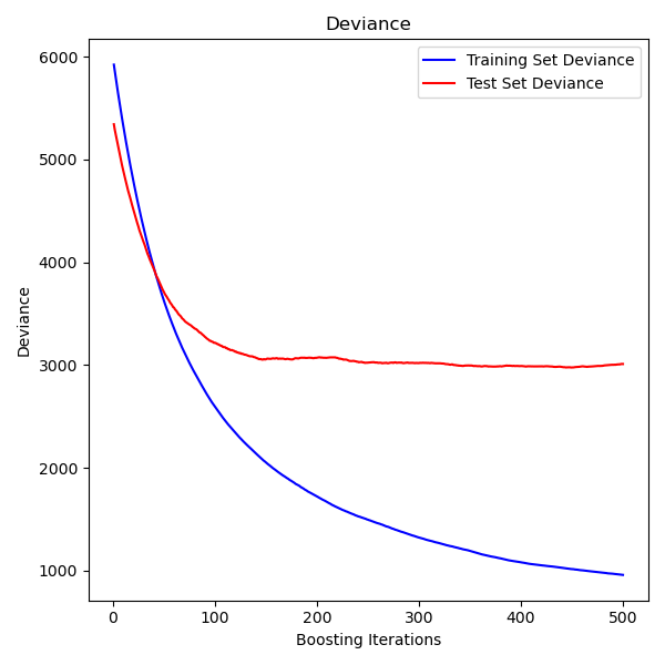
The figure below shows the results of applying GradientBoostingRegressor
with least squares loss and 500 base learners to the diabetes dataset
(sklearn.datasets.load_diabetes).
The plot shows the train and test error at each iteration.
The train error at each iteration is stored in the
train_score_ attribute of the gradient boosting model.
The test error at each iteration can be obtained
via the staged_predict method which returns a
generator that yields the predictions at each stage. Plots like these can be used
to determine the optimal number of trees (i.e. n_estimators) by early stopping.
Examples
1.11.1.2.1. Fitting additional weak-learners#
Both GradientBoostingRegressor and GradientBoostingClassifier
support warm_start=True which allows you to add more estimators to an already
fitted model.
>>> import numpy as np
>>> from sklearn.metrics import mean_squared_error
>>> from sklearn.datasets import make_friedman1
>>> from sklearn.ensemble import GradientBoostingRegressor

>>> X, y = make_friedman1(n_samples=1200, random_state=0, noise=1.0)
>>> X_train, X_test = X[:200], X[200:]
>>> y_train, y_test = y[:200], y[200:]
>>> est = GradientBoostingRegressor(
...     n_estimators=100, learning_rate=0.1, max_depth=1, random_state=0,
...     loss='squared_error'
... )
>>> est = est.fit(X_train, y_train)  # fit with 100 trees
>>> mean_squared_error(y_test, est.predict(X_test))
5.00
>>> _ = est.set_params(n_estimators=200, warm_start=True)  # set warm_start and increase num of trees
>>> _ = est.fit(X_train, y_train) # fit additional 100 trees to est
>>> mean_squared_error(y_test, est.predict(X_test))
3.84
1.11.1.2.2. Controlling the tree size#
The size of the regression tree base learners defines the level of variable
interactions that can be captured by the gradient boosting model. In general,
a tree of depth h can capture interactions of order h .
There are two ways in which the size of the individual regression trees can
be controlled.
If you specify max_depth=h then complete binary trees
of depth h will be grown. Such trees will have (at most) 2**h leaf nodes
and 2**h - 1 split nodes.
Alternatively, you can control the tree size by specifying the number of
leaf nodes via the parameter max_leaf_nodes. In this case,
trees will be grown using best-first search where nodes with the highest improvement
in impurity will be expanded first.
A tree with max_leaf_nodes=k has k - 1 split nodes and thus can
model interactions of up to order max_leaf_nodes - 1 .
We found that max_leaf_nodes=k gives comparable results to max_depth=k-1
but is significantly faster to train at the expense of a slightly higher
training error.
The parameter max_leaf_nodes corresponds to the variable J in the
chapter on gradient boosting in [Friedman2001] and is related to the parameter
interaction.depth in R’s gbm package where max_leaf_nodes == interaction.depth + 1 .
1.11.1.2.3. Mathematical formulation#
We first present GBRT for regression, and then detail the classification case.
Regression#
GBRT regressors are additive models whose prediction \(\hat{y}_i\) for a given input \(x_i\) is of the following form:
where the \(h_m\) are estimators called weak learners in the context
of boosting. Gradient Tree Boosting uses decision tree regressors of fixed size as weak learners. The constant M corresponds to the
n_estimators parameter.
Similar to other boosting algorithms, a GBRT is built in a greedy fashion:
where the newly added tree \(h_m\) is fitted in order to minimize a sum of losses \(L_m\), given the previous ensemble \(F_{m-1}\):
where \(l(y_i, F(x_i))\) is defined by the loss parameter, detailed
in the next section.
By default, the initial model \(F_{0}\) is chosen as the constant that
minimizes the loss: for a least-squares loss, this is the empirical mean of
the target values. The initial model can also be specified via the init
argument.
Using a first-order Taylor approximation, the value of \(l\) can be approximated as follows:
Note
Briefly, a first-order Taylor approximation says that \(l(z) \approx l(a) + (z - a) \frac{\partial l}{\partial z}(a)\). Here, \(z\) corresponds to \(F_{m - 1}(x_i) + h_m(x_i)\), and \(a\) corresponds to \(F_{m-1}(x_i)\)
The quantity \(\left[ \frac{\partial l(y_i, F(x_i))}{\partial F(x_i)} \right]_{F=F_{m - 1}}\) is the derivative of the loss with respect to its second parameter, evaluated at \(F_{m-1}(x)\). It is easy to compute for any given \(F_{m - 1}(x_i)\) in a closed form since the loss is differentiable. We will denote it by \(g_i\).
Removing the constant terms, we have:
This is minimized if \(h(x_i)\) is fitted to predict a value that is proportional to the negative gradient \(-g_i\). Therefore, at each iteration, the estimator \(h_m\) is fitted to predict the negative gradients of the samples. The gradients are updated at each iteration. This can be considered as some kind of gradient descent in a functional space.
Note
For some losses, e.g. 'absolute_error' where the gradients
are \(\pm 1\), the values predicted by a fitted \(h_m\) are not
accurate enough: the tree can only output integer values. As a result, the
leaves values of the tree \(h_m\) are modified once the tree is
fitted, such that the leaves values minimize the loss \(L_m\). The
update is loss-dependent: for the absolute error loss, the value of
a leaf is updated to the median of the samples in that leaf.
Classification#
Gradient boosting for classification is very similar to the regression case. However, the sum of the trees \(F_M(x_i) = \sum_m h_m(x_i)\) is not homogeneous to a prediction: it cannot be a class, since the trees predict continuous values.
The mapping from the value \(F_M(x_i)\) to a class or a probability is loss-dependent. For the log-loss, the probability that \(x_i\) belongs to the positive class is modeled as \(p(y_i = 1 | x_i) = \sigma(F_M(x_i))\) where \(\sigma\) is the sigmoid or expit function.
For multiclass classification, K trees (for K classes) are built at each of the \(M\) iterations. The probability that \(x_i\) belongs to class k is modeled as a softmax of the \(F_{M,k}(x_i)\) values.
Note that even for a classification task, the \(h_m\) sub-estimator is still a regressor, not a classifier. This is because the sub-estimators are trained to predict (negative) gradients, which are always continuous quantities.
1.11.1.2.4. Loss Functions#
The following loss functions are supported and can be specified using
the parameter loss:
Regression#
Squared error (
'squared_error'): The natural choice for regression due to its superior computational properties. The initial model is given by the mean of the target values.Absolute error (
'absolute_error'): A robust loss function for regression. The initial model is given by the median of the target values.Huber (
'huber'): Another robust loss function that combines least squares and least absolute deviation; usealphato control the sensitivity with regards to outliers (see [Friedman2001] for more details).Quantile (
'quantile'): A loss function for quantile regression. Use0 < alpha < 1to specify the quantile. This loss function can be used to create prediction intervals (see Prediction Intervals for Gradient Boosting Regression).
Classification#
Binary log-loss (
'log-loss'): The binomial negative log-likelihood loss function for binary classification. It provides probability estimates. The initial model is given by the log odds-ratio.Multi-class log-loss (
'log-loss'): The multinomial negative log-likelihood loss function for multi-class classification withn_classesmutually exclusive classes. It provides probability estimates. The initial model is given by the prior probability of each class. At each iterationn_classesregression trees have to be constructed which makes GBRT rather inefficient for data sets with a large number of classes.Exponential loss (
'exponential'): The same loss function asAdaBoostClassifier. Less robust to mislabeled examples than'log-loss'; can only be used for binary classification.
1.11.1.2.5. Shrinkage via learning rate#
[Friedman2001] proposed a simple regularization strategy that scales the contribution of each weak learner by a constant factor \(\nu\):
The parameter \(\nu\) is also called the learning rate because
it scales the step length of the gradient descent procedure; it can
be set via the learning_rate parameter.
The parameter learning_rate strongly interacts with the parameter
n_estimators, the number of weak learners to fit. Smaller values
of learning_rate require larger numbers of weak learners to maintain
a constant training error. Empirical evidence suggests that small
values of learning_rate favor better test error. [HTF]
recommend to set the learning rate to a small constant
(e.g. learning_rate <= 0.1) and choose n_estimators large enough
that early stopping applies,
see Early stopping in Gradient Boosting
for a more detailed discussion of the interaction between
learning_rate and n_estimators see [R2007].
1.11.1.2.6. Subsampling#
[Friedman2002] proposed stochastic gradient boosting, which combines gradient
boosting with bootstrap averaging (bagging). At each iteration
the base classifier is trained on a fraction subsample of
the available training data. The subsample is drawn without replacement.
A typical value of subsample is 0.5.
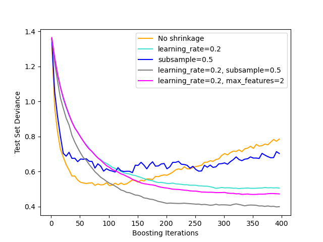
The figure below illustrates the effect of shrinkage and subsampling on the goodness-of-fit of the model. We can clearly see that shrinkage outperforms no-shrinkage. Subsampling with shrinkage can further increase the accuracy of the model. Subsampling without shrinkage, on the other hand, does poorly.
Another strategy to reduce the variance is by subsampling the features
analogous to the random splits in RandomForestClassifier.
The number of subsampled features can be controlled via the max_features
parameter.
Note
Using a small max_features value can significantly decrease the runtime.
Stochastic gradient boosting allows to compute out-of-bag estimates of the
test deviance by computing the improvement in deviance on the examples that are
not included in the bootstrap sample (i.e. the out-of-bag examples).
The improvements are stored in the attribute oob_improvement_.
oob_improvement_[i] holds the improvement in terms of the loss on the OOB samples
if you add the i-th stage to the current predictions.
Out-of-bag estimates can be used for model selection, for example to determine
the optimal number of iterations. OOB estimates are usually very pessimistic thus
we recommend to use cross-validation instead and only use OOB if cross-validation
is too time consuming.
Examples
1.11.1.2.7. Interpretation with feature importance#
Individual decision trees can be interpreted easily by simply visualizing the tree structure. Gradient boosting models, however, comprise hundreds of regression trees thus they cannot be easily interpreted by visual inspection of the individual trees. Fortunately, a number of techniques have been proposed to summarize and interpret gradient boosting models.
Often features do not contribute equally to predict the target response; in many situations the majority of the features are in fact irrelevant. When interpreting a model, the first question usually is: what are those important features and how do they contribute in predicting the target response?
Individual decision trees intrinsically perform feature selection by selecting appropriate split points. This information can be used to measure the importance of each feature; the basic idea is: the more often a feature is used in the split points of a tree the more important that feature is. This notion of importance can be extended to decision tree ensembles by simply averaging the impurity-based feature importance of each tree (see Feature importance evaluation for more details).
The feature importance scores of a fit gradient boosting model can be
accessed via the feature_importances_ property:
>>> from sklearn.datasets import make_hastie_10_2
>>> from sklearn.ensemble import GradientBoostingClassifier

>>> X, y = make_hastie_10_2(random_state=0)
>>> clf = GradientBoostingClassifier(n_estimators=100, learning_rate=1.0,
...     max_depth=1, random_state=0).fit(X, y)
>>> clf.feature_importances_
array([0.107, 0.105, 0.113, 0.0987, 0.0947,
       0.107, 0.0916, 0.0972, 0.0958, 0.0906])
Note that this computation of feature importance is based on entropy, and it
is distinct from sklearn.inspection.permutation_importance which is
based on permutation of the features.
Examples
References
Friedman, J.H. (2001). Greedy function approximation: A gradient boosting machine. Annals of Statistics, 29, 1189-1232.
Friedman, J.H. (2002). Stochastic gradient boosting.. Computational Statistics & Data Analysis, 38, 367-378.
G. Ridgeway (2006). Generalized Boosted Models: A guide to the gbm package
1.11.2. Random forests and other randomized tree ensembles#
The sklearn.ensemble module includes two averaging algorithms based
on randomized decision trees: the RandomForest algorithm
and the Extra-Trees method. Both algorithms are perturb-and-combine
techniques [B1998] specifically designed for trees. This means a diverse
set of classifiers is created by introducing randomness in the classifier
construction. The prediction of the ensemble is given as the averaged
prediction of the individual classifiers.
As other classifiers, forest classifiers have to be fitted with two
arrays: a sparse or dense array X of shape (n_samples, n_features)
holding the training samples, and an array Y of shape (n_samples,)
holding the target values (class labels) for the training samples:
>>> from sklearn.ensemble import RandomForestClassifier
>>> X = [[0, 0], [1, 1]]
>>> Y = [0, 1]
>>> clf = RandomForestClassifier(n_estimators=10)
>>> clf = clf.fit(X, Y)
Like decision trees, forests of trees also extend to
multi-output problems (if Y is an array
of shape (n_samples, n_outputs)).
1.11.2.1. Random Forests#
In random forests (see RandomForestClassifier and
RandomForestRegressor classes), each tree in the ensemble is built
from a sample drawn with replacement (i.e., a bootstrap sample) from the
training set.
During the construction of each tree in the forest, a random subset of the
features is considered. The size of this subset is controlled by the
max_features parameter; it may include either all input features or a random
subset of them (see the parameter tuning guidelines for more details).
The purpose of these two sources of randomness (bootstrapping the samples and randomly selecting features at each split) is to decrease the variance of the forest estimator. Indeed, individual decision trees typically exhibit high variance and tend to overfit. The injected randomness in forests yield decision trees with somewhat decoupled prediction errors. By taking an average of those predictions, some errors can cancel out. Random forests achieve a reduced variance by combining diverse trees, sometimes at the cost of a slight increase in bias. In practice the variance reduction is often significant hence yielding an overall better model.
When growing each tree in the forest, the “best” split (i.e. equivalent to
passing splitter="best" to the underlying decision trees) is chosen according
to the impurity criterion. See the CART mathematical formulation for more details.
In contrast to the original publication [B2001], the scikit-learn implementation combines classifiers by averaging their probabilistic prediction, instead of letting each classifier vote for a single class.
A competitive alternative to random forests are Histogram-Based Gradient Boosting (HGBT) models:
Building trees: Random forests typically rely on deep trees (that overfit individually) which uses much computational resources, as they require several splittings and evaluations of candidate splits. Boosting models build shallow trees (that underfit individually) which are faster to fit and predict.
Sequential boosting: In HGBT, the decision trees are built sequentially, where each tree is trained to correct the errors made by the previous ones. This allows them to iteratively improve the model’s performance using relatively few trees. In contrast, random forests use a majority vote to predict the outcome, which can require a larger number of trees to achieve the same level of accuracy.
Efficient binning: HGBT uses an efficient binning algorithm that can handle large datasets with a high number of features. The binning algorithm can pre-process the data to speed up the subsequent tree construction (see Why it’s faster). In contrast, the scikit-learn implementation of random forests does not use binning and relies on exact splitting, which can be computationally expensive.
Overall, the computational cost of HGBT versus RF depends on the specific characteristics of the dataset and the modeling task. It’s a good idea to try both models and compare their performance and computational efficiency on your specific problem to determine which model is the best fit.
Examples
1.11.2.2. Extremely Randomized Trees#
In extremely randomized trees (see ExtraTreesClassifier
and ExtraTreesRegressor classes), randomness goes one step
further in the way splits are computed. As in random forests, a random
subset of candidate features is used, but instead of looking for the
most discriminative thresholds, thresholds are drawn at random for each
candidate feature and the best of these randomly-generated thresholds is
picked as the splitting rule. This usually allows to reduce the variance
of the model a bit more, at the expense of a slightly greater increase
in bias:
>>> from sklearn.model_selection import cross_val_score
>>> from sklearn.datasets import make_blobs
>>> from sklearn.ensemble import RandomForestClassifier
>>> from sklearn.ensemble import ExtraTreesClassifier
>>> from sklearn.tree import DecisionTreeClassifier

>>> X, y = make_blobs(n_samples=10000, n_features=10, centers=100,
...     random_state=0)

>>> clf = DecisionTreeClassifier(max_depth=None, min_samples_split=2,
...     random_state=0)
>>> scores = cross_val_score(clf, X, y, cv=5)
>>> scores.mean()
np.float64(0.98)

>>> clf = RandomForestClassifier(n_estimators=10, max_depth=None,
...     min_samples_split=2, random_state=0)
>>> scores = cross_val_score(clf, X, y, cv=5)
>>> scores.mean()
np.float64(0.999)

>>> clf = ExtraTreesClassifier(n_estimators=10, max_depth=None,
...     min_samples_split=2, random_state=0)
>>> scores = cross_val_score(clf, X, y, cv=5)
>>> scores.mean() > 0.999
np.True_
1.11.2.3. Parameters#
The main parameters to adjust when using these methods is n_estimators and
max_features. The former is the number of trees in the forest. The larger
the better, but also the longer it will take to compute. In addition, note that
results will stop getting significantly better beyond a critical number of
trees. The latter is the size of the random subsets of features to consider
when splitting a node. The lower the greater the reduction of variance, but
also the greater the increase in bias. Empirical good default values are
max_features=1.0 or equivalently max_features=None (always considering
all features instead of a random subset) for regression problems, and
max_features="sqrt" (using a random subset of size sqrt(n_features))
for classification tasks (where n_features is the number of features in
the data). The default value of max_features=1.0 is equivalent to bagged
trees and more randomness can be achieved by setting smaller values (e.g. 0.3
is a typical default in the literature). Good results are often achieved when
setting max_depth=None in combination with min_samples_split=2 (i.e.,
when fully developing the trees). Bear in mind though that these values are
usually not optimal, and might result in models that consume a lot of RAM.
The best parameter values should always be cross-validated. In addition, note
that in random forests, bootstrap samples are used by default
(bootstrap=True) while the default strategy for extra-trees is to use the
whole dataset (bootstrap=False). When using bootstrap sampling the
generalization error can be estimated on the left out or out-of-bag samples.
This can be enabled by setting oob_score=True.
Note
The size of the model with the default parameters is \(O( M * N * log (N) )\),
where \(M\) is the number of trees and \(N\) is the number of samples.
In order to reduce the size of the model, you can change these parameters:
min_samples_split, max_leaf_nodes, max_depth and min_samples_leaf.
1.11.2.4. Parallelization#
Finally, this module also features the parallel construction of the trees
and the parallel computation of the predictions through the n_jobs
parameter. If n_jobs=k then computations are partitioned into
k jobs, and run on k cores of the machine. If n_jobs=-1
then all cores available on the machine are used. Note that because of
inter-process communication overhead, the speedup might not be linear
(i.e., using k jobs will unfortunately not be k times as
fast). Significant speedup can still be achieved though when building
a large number of trees, or when building a single tree requires a fair
amount of time (e.g., on large datasets).
Examples
References
Breiman, “Random Forests”, Machine Learning, 45(1), 5-32, 2001.
Breiman, “Arcing Classifiers”, Annals of Statistics 1998.
P. Geurts, D. Ernst., and L. Wehenkel, “Extremely randomized trees”, Machine Learning, 63(1), 3-42, 2006.
1.11.2.5. Feature importance evaluation#
The relative rank (i.e. depth) of a feature used as a decision node in a tree can be used to assess the relative importance of that feature with respect to the predictability of the target variable. Features used at the top of the tree contribute to the final prediction decision of a larger fraction of the input samples. The expected fraction of the samples they contribute to can thus be used as an estimate of the relative importance of the features. In scikit-learn, the fraction of samples a feature contributes to is combined with the decrease in impurity from splitting them to create a normalized estimate of the predictive power of that feature.
By averaging the estimates of predictive ability over several randomized trees one can reduce the variance of such an estimate and use it for feature selection. This is known as the mean decrease in impurity, or MDI. Refer to [L2014] for more information on MDI and feature importance evaluation with Random Forests.
Warning
The impurity-based feature importances computed on tree-based models suffer from two flaws that can lead to misleading conclusions. First they are computed on statistics derived from the training dataset and therefore do not necessarily inform us on which features are most important to make good predictions on held-out dataset. Secondly, they favor high cardinality features, that is features with many unique values. Permutation feature importance is an alternative to impurity-based feature importance that does not suffer from these flaws. These two methods of obtaining feature importance are explored in: Permutation Importance vs Random Forest Feature Importance (MDI).
In practice those estimates are stored as an attribute named
feature_importances_ on the fitted model. This is an array with shape
(n_features,) whose values are positive and sum to 1.0. The higher
the value, the more important is the contribution of the matching feature
to the prediction function.
Examples
References
G. Louppe, “Understanding Random Forests: From Theory to Practice”, PhD Thesis, U. of Liege, 2014.
1.11.2.6. Totally Random Trees Embedding#
RandomTreesEmbedding implements an unsupervised transformation of the
data. Using a forest of completely random trees, RandomTreesEmbedding
encodes the data by the indices of the leaves a data point ends up in. This
index is then encoded in a one-of-K manner, leading to a high dimensional,
sparse binary coding.
This coding can be computed very efficiently and can then be used as a basis
for other learning tasks.
The size and sparsity of the code can be influenced by choosing the number of
trees and the maximum depth per tree. For each tree in the ensemble, the coding
contains one entry of one. The size of the coding is at most n_estimators * 2
** max_depth, the maximum number of leaves in the forest.
As neighboring data points are more likely to lie within the same leaf of a tree, the transformation performs an implicit, non-parametric density estimation.
Examples
Manifold learning on handwritten digits: Locally Linear Embedding, Isomap… compares non-linear dimensionality reduction techniques on handwritten digits.
Feature transformations with ensembles of trees compares supervised and unsupervised tree based feature transformations.
See also
Manifold learning techniques can also be useful to derive non-linear representations of feature space, also these approaches focus also on dimensionality reduction.
1.11.2.7. Fitting additional trees#
RandomForest, Extra-Trees and RandomTreesEmbedding estimators all support
warm_start=True which allows you to add more trees to an already fitted model.
>>> from sklearn.datasets import make_classification
>>> from sklearn.ensemble import RandomForestClassifier

>>> X, y = make_classification(n_samples=100, random_state=1)
>>> clf = RandomForestClassifier(n_estimators=10)
>>> clf = clf.fit(X, y)  # fit with 10 trees
>>> len(clf.estimators_)
10
>>> # set warm_start and increase num of estimators
>>> _ = clf.set_params(n_estimators=20, warm_start=True)
>>> _ = clf.fit(X, y) # fit additional 10 trees
>>> len(clf.estimators_)
20
When random_state is also set, the internal random state is also preserved
between fit calls. This means that training a model once with n estimators is
the same as building the model iteratively via multiple fit calls, where the
final number of estimators is equal to n.
>>> clf = RandomForestClassifier(n_estimators=20)  # set `n_estimators` to 10 + 10
>>> _ = clf.fit(X, y)  # fit `estimators_` will be the same as `clf` above
Note that this differs from the usual behavior of random_state in that it does not result in the same result across different calls.
1.11.3. Bagging meta-estimator#
In ensemble algorithms, bagging methods form a class of algorithms which build several instances of a black-box estimator on random subsets of the original training set and then aggregate their individual predictions to form a final prediction. These methods are used as a way to reduce the variance of a base estimator (e.g., a decision tree), by introducing randomization into its construction procedure and then making an ensemble out of it. In many cases, bagging methods constitute a very simple way to improve with respect to a single model, without making it necessary to adapt the underlying base algorithm. As they provide a way to reduce overfitting, bagging methods work best with strong and complex models (e.g., fully developed decision trees), in contrast with boosting methods which usually work best with weak models (e.g., shallow decision trees).
Bagging methods come in many flavours but mostly differ from each other by the way they draw random subsets of the training set:
When random subsets of the dataset are drawn as random subsets of the samples, then this algorithm is known as Pasting [B1999].
When samples are drawn with replacement, then the method is known as Bagging [B1996].
When random subsets of the dataset are drawn as random subsets of the features, then the method is known as Random Subspaces [H1998].
Finally, when base estimators are built on subsets of both samples and features, then the method is known as Random Patches [LG2012].
In scikit-learn, bagging methods are offered as a unified
BaggingClassifier meta-estimator (resp. BaggingRegressor),
taking as input a user-specified estimator along with parameters
specifying the strategy to draw random subsets. In particular, max_samples
and max_features control the size of the subsets (in terms of samples and
features), while bootstrap and bootstrap_features control whether
samples and features are drawn with or without replacement. When using a subset
of the available samples the generalization accuracy can be estimated with the
out-of-bag samples by setting oob_score=True. As an example, the
snippet below illustrates how to instantiate a bagging ensemble of
KNeighborsClassifier estimators, each built on random
subsets of 50% of the samples and 50% of the features.
>>> from sklearn.ensemble import BaggingClassifier
>>> from sklearn.neighbors import KNeighborsClassifier
>>> bagging = BaggingClassifier(KNeighborsClassifier(),
...                             max_samples=0.5, max_features=0.5)
Examples
References
L. Breiman, “Pasting small votes for classification in large databases and on-line”, Machine Learning, 36(1), 85-103, 1999.
L. Breiman, “Bagging predictors”, Machine Learning, 24(2), 123-140, 1996.
T. Ho, “The random subspace method for constructing decision forests”, Pattern Analysis and Machine Intelligence, 20(8), 832-844, 1998.
G. Louppe and P. Geurts, “Ensembles on Random Patches”, Machine Learning and Knowledge Discovery in Databases, 346-361, 2012.
1.11.4. Voting Classifier#
The idea behind the VotingClassifier is to combine
conceptually different machine learning classifiers and use a majority vote
or the average predicted probabilities (soft vote) to predict the class labels.
Such a classifier can be useful for a set of equally well performing models
in order to balance out their individual weaknesses.
1.11.4.1. Majority Class Labels (Majority/Hard Voting)#
In majority voting, the predicted class label for a particular sample is the class label that represents the majority (mode) of the class labels predicted by each individual classifier.
E.g., if the prediction for a given sample is
classifier 1 -> class 1
classifier 2 -> class 1
classifier 3 -> class 2
the VotingClassifier (with voting='hard') would classify the sample
as “class 1” based on the majority class label.
In the cases of a tie, the VotingClassifier will select the class
based on the ascending sort order. E.g., in the following scenario
classifier 1 -> class 2
classifier 2 -> class 1
the class label 1 will be assigned to the sample.
1.11.4.2. Usage#
The following example shows how to fit the majority rule classifier:
>>> from sklearn import datasets
>>> from sklearn.model_selection import cross_val_score
>>> from sklearn.linear_model import LogisticRegression
>>> from sklearn.naive_bayes import GaussianNB
>>> from sklearn.ensemble import RandomForestClassifier
>>> from sklearn.ensemble import VotingClassifier

>>> iris = datasets.load_iris()
>>> X, y = iris.data[:, 1:3], iris.target

>>> clf1 = LogisticRegression(random_state=1)
>>> clf2 = RandomForestClassifier(n_estimators=50, random_state=1)
>>> clf3 = GaussianNB()

>>> eclf = VotingClassifier(
...     estimators=[('lr', clf1), ('rf', clf2), ('gnb', clf3)],
...     voting='hard')

>>> for clf, label in zip([clf1, clf2, clf3, eclf], ['Logistic Regression', 'Random Forest', 'naive Bayes', 'Ensemble']):
...     scores = cross_val_score(clf, X, y, scoring='accuracy', cv=5)
...     print("Accuracy: %0.2f (+/- %0.2f) [%s]" % (scores.mean(), scores.std(), label))
Accuracy: 0.95 (+/- 0.04) [Logistic Regression]
Accuracy: 0.94 (+/- 0.04) [Random Forest]
Accuracy: 0.91 (+/- 0.04) [naive Bayes]
Accuracy: 0.95 (+/- 0.04) [Ensemble]
1.11.4.3. Weighted Average Probabilities (Soft Voting)#
In contrast to majority voting (hard voting), soft voting returns the class label as argmax of the sum of predicted probabilities.
Specific weights can be assigned to each classifier via the weights
parameter. When weights are provided, the predicted class probabilities
for each classifier are collected, multiplied by the classifier weight,
and averaged. The final class label is then derived from the class label
with the highest average probability.
To illustrate this with a simple example, let’s assume we have 3 classifiers and a 3-class classification problem where we assign equal weights to all classifiers: w1=1, w2=1, w3=1.
The weighted average probabilities for a sample would then be calculated as follows:
classifier |
class 1 |
class 2 |
class 3 |
|---|---|---|---|
classifier 1 |
w1 * 0.2 |
w1 * 0.5 |
w1 * 0.3 |
classifier 2 |
w2 * 0.6 |
w2 * 0.3 |
w2 * 0.1 |
classifier 3 |
w3 * 0.3 |
w3 * 0.4 |
w3 * 0.3 |
weighted average |
0.37 |
0.4 |
0.23 |
Here, the predicted class label is 2, since it has the highest average predicted probability. See the example on Visualizing the probabilistic predictions of a VotingClassifier for a demonstration of how the predicted class label can be obtained from the weighted average of predicted probabilities.
The following figure illustrates how the decision regions may change when
a soft VotingClassifier is trained with weights on three linear
models:
1.11.4.4. Usage#
In order to predict the class labels based on the predicted
class-probabilities (scikit-learn estimators in the VotingClassifier
must support predict_proba method):
>>> eclf = VotingClassifier(
...     estimators=[('lr', clf1), ('rf', clf2), ('gnb', clf3)],
...     voting='soft'
... )
Optionally, weights can be provided for the individual classifiers:
>>> eclf = VotingClassifier(
...     estimators=[('lr', clf1), ('rf', clf2), ('gnb', clf3)],
...     voting='soft', weights=[2,5,1]
... )
Using the VotingClassifier with GridSearchCV#
The VotingClassifier can also be used together with
GridSearchCV in order to tune the
hyperparameters of the individual estimators:
>>> from sklearn.model_selection import GridSearchCV
>>> clf1 = LogisticRegression(random_state=1)
>>> clf2 = RandomForestClassifier(random_state=1)
>>> clf3 = GaussianNB()
>>> eclf = VotingClassifier(
...     estimators=[('lr', clf1), ('rf', clf2), ('gnb', clf3)],
...     voting='soft'
... )

>>> params = {'lr__C': [1.0, 100.0], 'rf__n_estimators': [20, 200]}

>>> grid = GridSearchCV(estimator=eclf, param_grid=params, cv=5)
>>> grid = grid.fit(iris.data, iris.target)
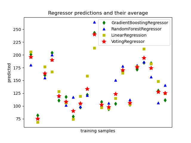
1.11.5. Voting Regressor#
The idea behind the VotingRegressor is to combine conceptually
different machine learning regressors and return the average predicted values.
Such a regressor can be useful for a set of equally well performing models
in order to balance out their individual weaknesses.
1.11.5.1. Usage#
The following example shows how to fit the VotingRegressor:
>>> from sklearn.datasets import load_diabetes
>>> from sklearn.ensemble import GradientBoostingRegressor
>>> from sklearn.ensemble import RandomForestRegressor
>>> from sklearn.linear_model import LinearRegression
>>> from sklearn.ensemble import VotingRegressor

>>> # Loading some example data
>>> X, y = load_diabetes(return_X_y=True)

>>> # Training classifiers
>>> reg1 = GradientBoostingRegressor(random_state=1)
>>> reg2 = RandomForestRegressor(random_state=1)
>>> reg3 = LinearRegression()
>>> ereg = VotingRegressor(estimators=[('gb', reg1), ('rf', reg2), ('lr', reg3)])
>>> ereg = ereg.fit(X, y)
Examples
1.11.6. Stacked generalization#
Stacked generalization is a method for combining estimators to reduce their biases [W1992] [HTF]. More precisely, the predictions of each individual estimator are stacked together and used as input to a final estimator to compute the prediction. This final estimator is trained through cross-validation.
The StackingClassifier and StackingRegressor provide such
strategies which can be applied to classification and regression problems.
The estimators parameter corresponds to the list of the estimators which
are stacked together in parallel on the input data. It should be given as a
list of names and estimators:
>>> from sklearn.linear_model import RidgeCV, LassoCV
>>> from sklearn.neighbors import KNeighborsRegressor
>>> estimators = [('ridge', RidgeCV()),
...               ('lasso', LassoCV(random_state=42)),
...               ('knr', KNeighborsRegressor(n_neighbors=20,
...                                           metric='euclidean'))]
The final_estimator will use the predictions of the estimators as input. It
needs to be a classifier or a regressor when using StackingClassifier
or StackingRegressor, respectively:
>>> from sklearn.ensemble import GradientBoostingRegressor
>>> from sklearn.ensemble import StackingRegressor
>>> final_estimator = GradientBoostingRegressor(
...     n_estimators=25, subsample=0.5, min_samples_leaf=25, max_features=1,
...     random_state=42)
>>> reg = StackingRegressor(
...     estimators=estimators,
...     final_estimator=final_estimator)
To train the estimators and final_estimator, the fit method needs
to be called on the training data:
>>> from sklearn.datasets import load_diabetes
>>> X, y = load_diabetes(return_X_y=True)
>>> from sklearn.model_selection import train_test_split
>>> X_train, X_test, y_train, y_test = train_test_split(X, y,
...                                                     random_state=42)
>>> reg.fit(X_train, y_train)
StackingRegressor(...)
During training, the estimators are fitted on the whole training data
X_train. They will be used when calling predict or predict_proba. To
generalize and avoid over-fitting, the final_estimator is trained on
out-samples using sklearn.model_selection.cross_val_predict internally.
For StackingClassifier, note that the output of the estimators is
controlled by the parameter stack_method and it is called by each estimator.
This parameter is either a string, being estimator method names, or 'auto'
which will automatically identify an available method depending on the
availability, tested in the order of preference: predict_proba,
decision_function and predict.
A StackingRegressor and StackingClassifier can be used as
any other regressor or classifier, exposing a predict, predict_proba, or
decision_function method, e.g.:
>>> y_pred = reg.predict(X_test)
>>> from sklearn.metrics import r2_score
>>> print('R2 score: {:.2f}'.format(r2_score(y_test, y_pred)))
R2 score: 0.53
Note that it is also possible to get the output of the stacked
estimators using the transform method:
>>> reg.transform(X_test[:5])
array([[142, 138, 146],
       [179, 182, 151],
       [139, 132, 158],
       [286, 292, 225],
       [126, 124, 164]])
In practice, a stacking predictor predicts as good as the best predictor of the base layer and even sometimes outperforms it by combining the different strengths of these predictors. However, training a stacking predictor is computationally expensive.
Note
For StackingClassifier, when using stack_method_='predict_proba',
the first column is dropped when the problem is a binary classification
problem. Indeed, both probability columns predicted by each estimator are
perfectly collinear.
Note
Multiple stacking layers can be achieved by assigning final_estimator to
a StackingClassifier or StackingRegressor:
>>> final_layer_rfr = RandomForestRegressor(
...     n_estimators=10, max_features=1, max_leaf_nodes=5,random_state=42)
>>> final_layer_gbr = GradientBoostingRegressor(
...     n_estimators=10, max_features=1, max_leaf_nodes=5,random_state=42)
>>> final_layer = StackingRegressor(
...     estimators=[('rf', final_layer_rfr),
...                 ('gbrt', final_layer_gbr)],
...     final_estimator=RidgeCV()
...     )
>>> multi_layer_regressor = StackingRegressor(
...     estimators=[('ridge', RidgeCV()),
...                 ('lasso', LassoCV(random_state=42)),
...                 ('knr', KNeighborsRegressor(n_neighbors=20,
...                                             metric='euclidean'))],
...     final_estimator=final_layer
... )
>>> multi_layer_regressor.fit(X_train, y_train)
StackingRegressor(...)
>>> print('R2 score: {:.2f}'
...       .format(multi_layer_regressor.score(X_test, y_test)))
R2 score: 0.53
Examples
References
Wolpert, David H. “Stacked generalization.” Neural networks 5.2 (1992): 241-259.
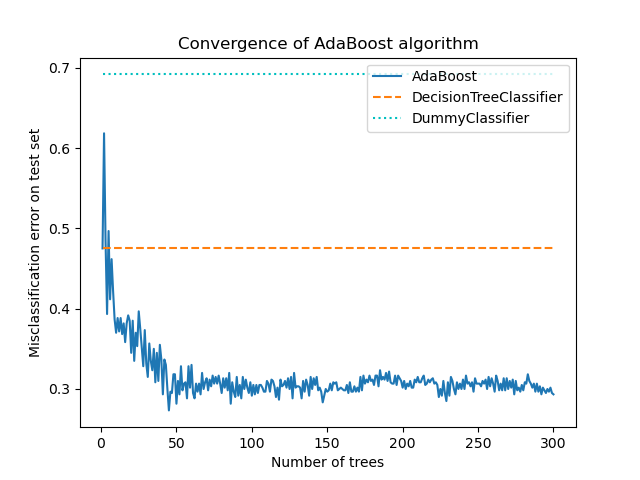
1.11.7. AdaBoost#
The module sklearn.ensemble includes the popular boosting algorithm
AdaBoost, introduced in 1995 by Freund and Schapire [FS1995].
The core principle of AdaBoost is to fit a sequence of weak learners (i.e., models that are only slightly better than random guessing, such as small decision trees) on repeatedly modified versions of the data. The predictions from all of them are then combined through a weighted majority vote (or sum) to produce the final prediction. The data modifications at each so-called boosting iteration consists of applying weights \(w_1\), \(w_2\), …, \(w_N\) to each of the training samples. Initially, those weights are all set to \(w_i = 1/N\), so that the first step simply trains a weak learner on the original data. For each successive iteration, the sample weights are individually modified and the learning algorithm is reapplied to the reweighted data. At a given step, those training examples that were incorrectly predicted by the boosted model induced at the previous step have their weights increased, whereas the weights are decreased for those that were predicted correctly. As iterations proceed, examples that are difficult to predict receive ever-increasing influence. Each subsequent weak learner is thereby forced to concentrate on the examples that are missed by the previous ones in the sequence [HTF].
AdaBoost can be used both for classification and regression problems:
For multi-class classification,
AdaBoostClassifierimplements AdaBoost.SAMME [ZZRH2009].For regression,
AdaBoostRegressorimplements AdaBoost.R2 [D1997].
1.11.7.1. Usage#
The following example shows how to fit an AdaBoost classifier with 100 weak learners:
>>> from sklearn.model_selection import cross_val_score
>>> from sklearn.datasets import load_iris
>>> from sklearn.ensemble import AdaBoostClassifier

>>> X, y = load_iris(return_X_y=True)
>>> clf = AdaBoostClassifier(n_estimators=100)
>>> scores = cross_val_score(clf, X, y, cv=5)
>>> scores.mean()
np.float64(0.95)
The number of weak learners is controlled by the parameter n_estimators. The
learning_rate parameter controls the contribution of the weak learners in
the final combination. By default, weak learners are decision stumps. Different
weak learners can be specified through the estimator parameter.
The main parameters to tune to obtain good results are n_estimators and
the complexity of the base estimators (e.g., its depth max_depth or
minimum required number of samples to consider a split min_samples_split).
Examples
Multi-class AdaBoosted Decision Trees shows the performance of AdaBoost on a multi-class problem.
Two-class AdaBoost shows the decision boundary and decision function values for a non-linearly separable two-class problem using AdaBoost-SAMME.
Decision Tree Regression with AdaBoost demonstrates regression with the AdaBoost.R2 algorithm.
References
