2.7. Novelty and Outlier Detection#
Many applications require being able to decide whether a new observation belongs to the same distribution as existing observations (it is an inlier), or should be considered as different (it is an outlier). Often, this ability is used to clean real data sets. Two important distinctions must be made:
- outlier detection:
The training data contains outliers which are defined as observations that are far from the others. Outlier detection estimators thus try to fit the regions where the training data is the most concentrated, ignoring the deviant observations.
- novelty detection:
The training data is not polluted by outliers and we are interested in detecting whether a new observation is an outlier. In this context an outlier is also called a novelty.
Outlier detection and novelty detection are both used for anomaly detection, where one is interested in detecting abnormal or unusual observations. Outlier detection is then also known as unsupervised anomaly detection and novelty detection as semi-supervised anomaly detection. In the context of outlier detection, the outliers/anomalies cannot form a dense cluster as available estimators assume that the outliers/anomalies are located in low density regions. On the contrary, in the context of novelty detection, novelties/anomalies can form a dense cluster as long as they are in a low density region of the training data, considered as normal in this context.
The scikit-learn project provides a set of machine learning tools that can be used both for novelty or outlier detection. This strategy is implemented with objects learning in an unsupervised way from the data:
estimator.fit(X_train)
new observations can then be sorted as inliers or outliers with a
predict method:
estimator.predict(X_test)
Inliers are labeled 1, while outliers are labeled -1. The predict method
makes use of a threshold on the raw scoring function computed by the
estimator. This scoring function is accessible through the score_samples
method, while the threshold can be controlled by the contamination
parameter.
The decision_function method is also defined from the scoring function,
in such a way that negative values are outliers and non-negative ones are
inliers:
estimator.decision_function(X_test)
Note that neighbors.LocalOutlierFactor does not support
predict, decision_function and score_samples methods by default
but only a fit_predict method, as this estimator was originally meant to
be applied for outlier detection. The scores of abnormality of the training
samples are accessible through the negative_outlier_factor_ attribute.
If you really want to use neighbors.LocalOutlierFactor for novelty
detection, i.e. predict labels or compute the score of abnormality of new
unseen data, you can instantiate the estimator with the novelty parameter
set to True before fitting the estimator. In this case, fit_predict is
not available.
Warning
Novelty detection with Local Outlier Factor
When novelty is set to True be aware that you must only use
predict, decision_function and score_samples on new unseen data
and not on the training samples as this would lead to wrong results.
I.e., the result of predict will not be the same as fit_predict.
The scores of abnormality of the training samples are always accessible
through the negative_outlier_factor_ attribute.
The behavior of neighbors.LocalOutlierFactor is summarized in the
following table.
Method |
Outlier detection |
Novelty detection |
|---|---|---|
|
OK |
Not available |
|
Not available |
Use only on new data |
|
Not available |
Use only on new data |
|
Use |
Use only on new data |
|
OK |
OK |
2.7.1. Overview of outlier detection methods#
A comparison of the outlier detection algorithms in scikit-learn. Local Outlier Factor (LOF) does not show a decision boundary in black as it has no predict method to be applied on new data when it is used for outlier detection.
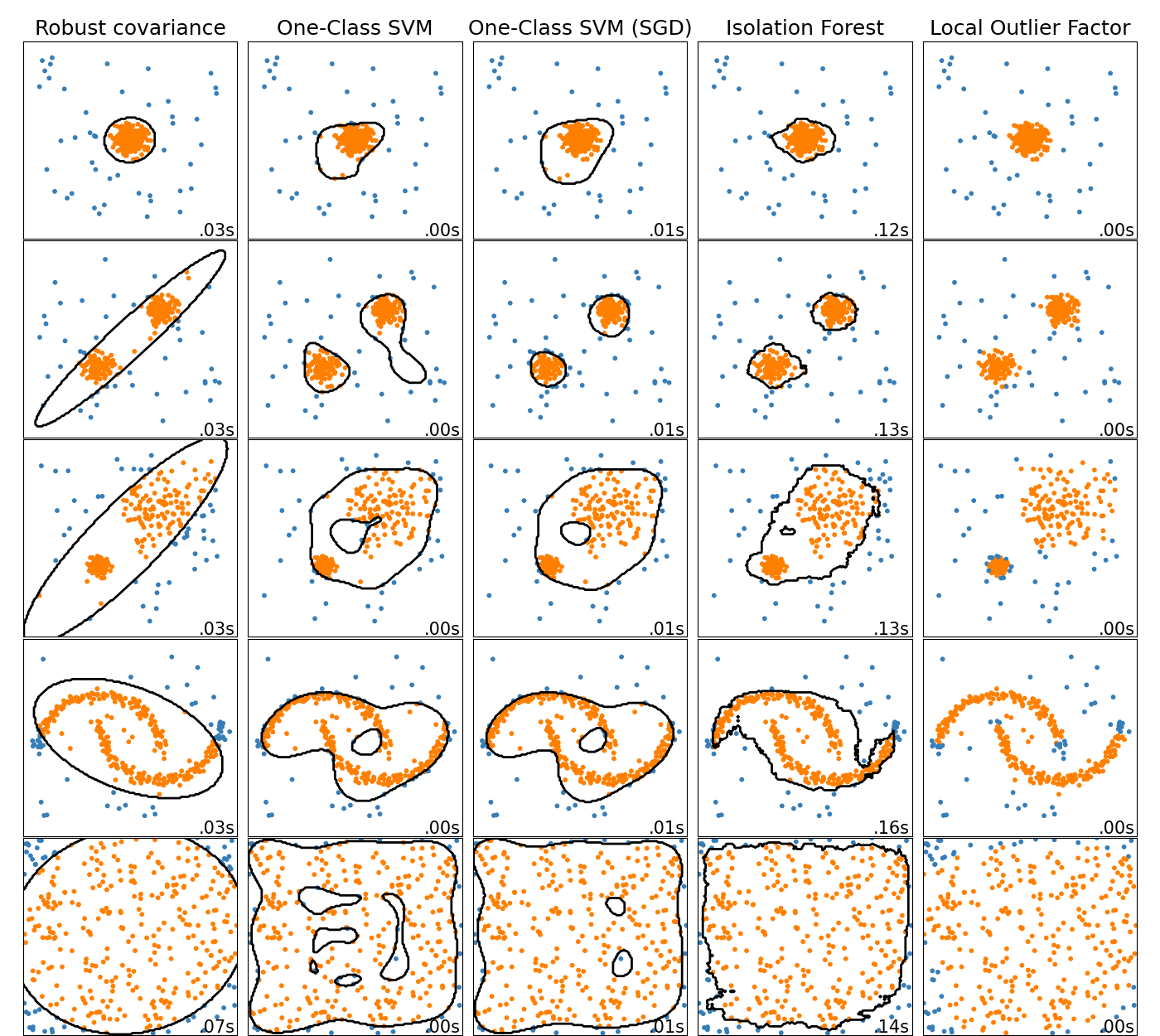
ensemble.IsolationForest and neighbors.LocalOutlierFactor
perform reasonably well on the data sets considered here.
The svm.OneClassSVM is known to be sensitive to outliers and thus
does not perform very well for outlier detection. That being said, outlier
detection in high-dimension, or without any assumptions on the distribution
of the inlying data is very challenging. svm.OneClassSVM may still
be used with outlier detection but requires fine-tuning of its hyperparameter
nu to handle outliers and prevent overfitting.
linear_model.SGDOneClassSVM provides an implementation of a
linear One-Class SVM with a linear complexity in the number of samples. This
implementation is here used with a kernel approximation technique to obtain
results similar to svm.OneClassSVM which uses a Gaussian kernel
by default. Finally, covariance.EllipticEnvelope assumes the data is
Gaussian and learns an ellipse. For more details on the different estimators
refer to the example
Comparing anomaly detection algorithms for outlier detection on toy datasets and the
sections hereunder.
Examples
See Comparing anomaly detection algorithms for outlier detection on toy datasets for a comparison of the
svm.OneClassSVM, theensemble.IsolationForest, theneighbors.LocalOutlierFactorandcovariance.EllipticEnvelope.See Evaluation of outlier detection estimators for an example showing how to evaluate outlier detection estimators, the
neighbors.LocalOutlierFactorand theensemble.IsolationForest, using ROC curves frommetrics.RocCurveDisplay.
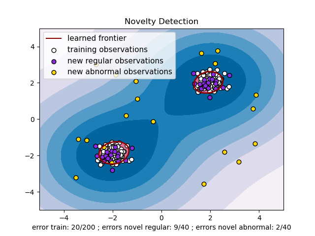
2.7.2. Novelty Detection#
Consider a data set of \(n\) observations from the same distribution described by \(p\) features. Consider now that we add one more observation to that data set. Is the new observation so different from the others that we can doubt it is regular? (i.e. does it come from the same distribution?) Or on the contrary, is it so similar to the other that we cannot distinguish it from the original observations? This is the question addressed by the novelty detection tools and methods.
In general, it is about to learn a rough, close frontier delimiting the contour of the initial observations distribution, plotted in embedding \(p\)-dimensional space. Then, if further observations lay within the frontier-delimited subspace, they are considered as coming from the same population as the initial observations. Otherwise, if they lay outside the frontier, we can say that they are abnormal with a given confidence in our assessment.
The One-Class SVM has been introduced by Schölkopf et al. for that purpose
and implemented in the Support Vector Machines module in the
svm.OneClassSVM object. It requires the choice of a
kernel and a scalar parameter to define a frontier. The RBF kernel is
usually chosen although there exists no exact formula or algorithm to
set its bandwidth parameter. This is the default in the scikit-learn
implementation. The nu parameter, also known as the margin of
the One-Class SVM, corresponds to the probability of finding a new,
but regular, observation outside the frontier.
References
Estimating the support of a high-dimensional distribution Schölkopf, Bernhard, et al. Neural computation 13.7 (2001): 1443-1471.
Examples
See One-class SVM with non-linear kernel (RBF) for visualizing the frontier learned around some data by a
svm.OneClassSVMobject.
2.7.2.1. Scaling up the One-Class SVM#
An online linear version of the One-Class SVM is implemented in
linear_model.SGDOneClassSVM. This implementation scales linearly with
the number of samples and can be used with a kernel approximation to
approximate the solution of a kernelized svm.OneClassSVM whose
complexity is at best quadratic in the number of samples. See section
Online One-Class SVM for more details.
Examples
See One-Class SVM versus One-Class SVM using Stochastic Gradient Descent for an illustration of the approximation of a kernelized One-Class SVM with the
linear_model.SGDOneClassSVMcombined with kernel approximation.
2.7.3. Outlier Detection#
Outlier detection is similar to novelty detection in the sense that the goal is to separate a core of regular observations from some polluting ones, called outliers. Yet, in the case of outlier detection, we don’t have a clean data set representing the population of regular observations that can be used to train any tool.
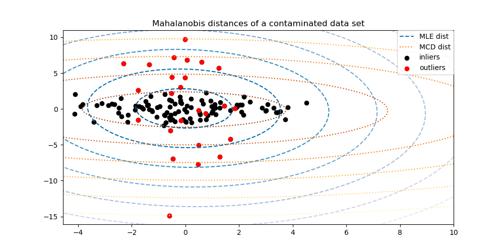
2.7.3.1. Fitting an elliptic envelope#
One common way of performing outlier detection is to assume that the regular data come from a known distribution (e.g. data are Gaussian distributed). From this assumption, we generally try to define the “shape” of the data, and can define outlying observations as observations which stand far enough from the fit shape.
The scikit-learn provides an object
covariance.EllipticEnvelope that fits a robust covariance
estimate to the data, and thus fits an ellipse to the central data
points, ignoring points outside the central mode.
For instance, assuming that the inlier data are Gaussian distributed, it will estimate the inlier location and covariance in a robust way (i.e. without being influenced by outliers). The Mahalanobis distances obtained from this estimate are used to derive a measure of outlyingness. This strategy is illustrated below.
Examples
See Robust covariance estimation and Mahalanobis distances relevance for an illustration of the difference between using a standard (
covariance.EmpiricalCovariance) or a robust estimate (covariance.MinCovDet) of location and covariance to assess the degree of outlyingness of an observation.See Outlier detection on a real data set for an example of robust covariance estimation on a real data set.
References
Rousseeuw, P.J., Van Driessen, K. “A fast algorithm for the minimum covariance determinant estimator” Technometrics 41(3), 212 (1999)
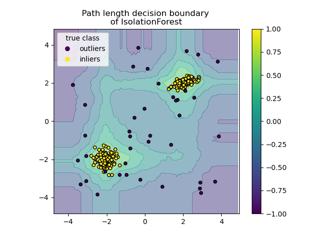
2.7.3.2. Isolation Forest#
One efficient way of performing outlier detection in high-dimensional datasets
is to use random forests.
The ensemble.IsolationForest ‘isolates’ observations by randomly selecting
a feature and then randomly selecting a split value between the maximum and
minimum values of the selected feature.
Since recursive partitioning can be represented by a tree structure, the number of splittings required to isolate a sample is equivalent to the path length from the root node to the terminating node.
This path length, averaged over a forest of such random trees, is a measure of normality and our decision function.
Random partitioning produces noticeably shorter paths for anomalies. Hence, when a forest of random trees collectively produce shorter path lengths for particular samples, they are highly likely to be anomalies.
The implementation of ensemble.IsolationForest is based on an ensemble
of tree.ExtraTreeRegressor. Following Isolation Forest original paper,
the maximum depth of each tree is set to \(\lceil \log_2(n) \rceil\) where
\(n\) is the number of samples used to build the tree (see [1]
for more details).
This algorithm is illustrated below.
The ensemble.IsolationForest supports warm_start=True which
allows you to add more trees to an already fitted model:
>>> from sklearn.ensemble import IsolationForest
>>> import numpy as np
>>> X = np.array([[-1, -1], [-2, -1], [-3, -2], [0, 0], [-20, 50], [3, 5]])
>>> clf = IsolationForest(n_estimators=10, warm_start=True)
>>> clf.fit(X)  # fit 10 trees
>>> clf.set_params(n_estimators=20)  # add 10 more trees
>>> clf.fit(X)  # fit the added trees
Examples
See IsolationForest example for an illustration of the use of IsolationForest.
See Comparing anomaly detection algorithms for outlier detection on toy datasets for a comparison of
ensemble.IsolationForestwithneighbors.LocalOutlierFactor,svm.OneClassSVM(tuned to perform like an outlier detection method),linear_model.SGDOneClassSVM, and a covariance-based outlier detection withcovariance.EllipticEnvelope.
References
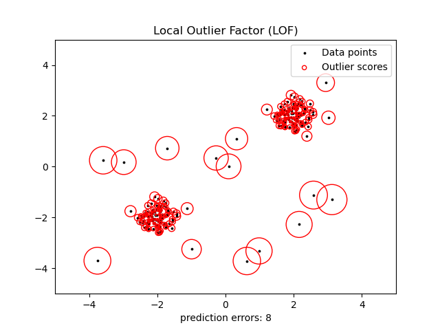
2.7.3.3. Local Outlier Factor#
Another efficient way to perform outlier detection on moderately high dimensional datasets is to use the Local Outlier Factor (LOF) algorithm.
The neighbors.LocalOutlierFactor (LOF) algorithm computes a score
(called local outlier factor) reflecting the degree of abnormality of the
observations.
It measures the local density deviation of a given data point with respect to
its neighbors. The idea is to detect the samples that have a substantially
lower density than their neighbors.
In practice the local density is obtained from the k-nearest neighbors. The LOF score of an observation is equal to the ratio of the average local density of its k-nearest neighbors, and its own local density: a normal instance is expected to have a local density similar to that of its neighbors, while abnormal data are expected to have much smaller local density.
The number k of neighbors considered, (alias parameter n_neighbors) is
typically chosen 1) greater than the minimum number of objects a cluster has to
contain, so that other objects can be local outliers relative to this cluster,
and 2) smaller than the maximum number of close by objects that can potentially
be local outliers. In practice, such information is generally not available, and
taking n_neighbors=20 appears to work well in general. When the proportion of
outliers is high (i.e. greater than 10 %, as in the example below),
n_neighbors should be greater (n_neighbors=35 in the example below).
The strength of the LOF algorithm is that it takes both local and global properties of datasets into consideration: it can perform well even in datasets where abnormal samples have different underlying densities. The question is not, how isolated the sample is, but how isolated it is with respect to the surrounding neighborhood.
When applying LOF for outlier detection, there are no predict,
decision_function and score_samples methods but only a fit_predict
method. The scores of abnormality of the training samples are accessible
through the negative_outlier_factor_ attribute.
Note that predict, decision_function and score_samples can be used
on new unseen data when LOF is applied for novelty detection, i.e. when the
novelty parameter is set to True, but the result of predict may
differ from that of fit_predict. See Novelty detection with Local Outlier Factor.
When the contamination parameter is set, the threshold (called offset_)
is determined as the corresponding percentile of negative_outlier_factor_
scores on the training data. Samples with scores strictly below this threshold
are classified as outliers.
This strategy is illustrated below.
Examples
See Outlier detection with Local Outlier Factor (LOF) for an illustration of the use of
neighbors.LocalOutlierFactor.See Comparing anomaly detection algorithms for outlier detection on toy datasets for a comparison with other anomaly detection methods.
References
Breunig, Kriegel, Ng, and Sander (2000) LOF: identifying density-based local outliers. Proc. ACM SIGMOD
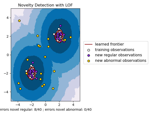
2.7.4. Novelty detection with Local Outlier Factor#
To use neighbors.LocalOutlierFactor for novelty detection, i.e.
predict labels or compute the score of abnormality of new unseen data, you
need to instantiate the estimator with the novelty parameter
set to True before fitting the estimator:
lof = LocalOutlierFactor(novelty=True)
lof.fit(X_train)
Note that fit_predict is not available in this case to avoid inconsistencies.
Warning
Novelty detection with Local Outlier Factor
When novelty is set to True be aware that you must only use
predict, decision_function and score_samples on new unseen data
and not on the training samples as this would lead to wrong results.
I.e., the result of predict will not be the same as fit_predict.
The scores of abnormality of the training samples are always accessible
through the negative_outlier_factor_ attribute.
Novelty detection with neighbors.LocalOutlierFactor is illustrated below
(see Novelty detection with Local Outlier Factor (LOF)).