LocalOutlierFactor#
- class sklearn.neighbors.LocalOutlierFactor(n_neighbors=20, *, algorithm='auto', leaf_size=30, metric='minkowski', p=2, metric_params=None, contamination='auto', novelty=False, n_jobs=None)[source]#
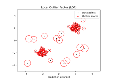
Unsupervised Outlier Detection using the Local Outlier Factor (LOF).
The anomaly score of each sample is called the Local Outlier Factor. It measures the local deviation of the density of a given sample with respect to its neighbors. It is local in that the anomaly score depends on how isolated the object is with respect to the surrounding neighborhood. More precisely, locality is given by k-nearest neighbors, whose distance is used to estimate the local density. By comparing the local density of a sample to the local densities of its neighbors, one can identify samples that have a substantially lower density than their neighbors. These are considered outliers.
Read more in the User Guide.
Added in version 0.19.
- Parameters:
- n_neighborsint, default=20
Number of neighbors to use by default for
kneighborsqueries. If n_neighbors is larger than the number of samples provided, all samples will be used.- algorithm{‘auto’, ‘ball_tree’, ‘kd_tree’, ‘brute’}, default=’auto’
Algorithm used to compute the nearest neighbors:
‘ball_tree’ will use
BallTree‘kd_tree’ will use
KDTree‘brute’ will use a brute-force search.
‘auto’ will attempt to decide the most appropriate algorithm based on the values passed to
fitmethod.
Note: fitting on sparse input will override the setting of this parameter, using brute force.
- leaf_sizeint, default=30
Leaf is size passed to
BallTreeorKDTree. This can affect the speed of the construction and query, as well as the memory required to store the tree. The optimal value depends on the nature of the problem.- metricstr or callable, default=’minkowski’
Metric to use for distance computation. Default is “minkowski”, which results in the standard Euclidean distance when p = 2. See the documentation of scipy.spatial.distance and the metrics listed in
distance_metricsfor valid metric values.If metric is “precomputed”, X is assumed to be a distance matrix and must be square during fit. X may be a sparse graph, in which case only “nonzero” elements may be considered neighbors.
If metric is a callable function, it takes two arrays representing 1D vectors as inputs and must return one value indicating the distance between those vectors. This works for Scipy’s metrics, but is less efficient than passing the metric name as a string.
- pfloat, default=2
Parameter for the Minkowski metric from
sklearn.metrics.pairwise_distances. When p = 1, this is equivalent to using manhattan_distance (l1), and euclidean_distance (l2) for p = 2. For arbitrary p, minkowski_distance (l_p) is used.- metric_paramsdict, default=None
Additional keyword arguments for the metric function.
- contamination‘auto’ or float, default=’auto’
The amount of contamination of the data set, i.e. the proportion of outliers in the data set. When fitting this is used to define the threshold on the scores of the samples.
if ‘auto’, the threshold is determined as in the original paper,
if a float, the contamination should be in the range (0, 0.5].
Changed in version 0.22: The default value of
contaminationchanged from 0.1 to'auto'.- noveltybool, default=False
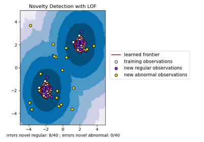
By default, LocalOutlierFactor is only meant to be used for outlier detection (novelty=False). Set novelty to True if you want to use LocalOutlierFactor for novelty detection. In this case be aware that you should only use predict, decision_function and score_samples on new unseen data and not on the training set; and note that the results obtained this way may differ from the standard LOF results.
Added in version 0.20.
- n_jobsint, default=None
The number of parallel jobs to run for neighbors search.
Nonemeans 1 unless in ajoblib.parallel_backendcontext.-1means using all processors. See Glossary for more details.
- Attributes:
- negative_outlier_factor_ndarray of shape (n_samples,)
The opposite LOF of the training samples. The higher, the more normal. Inliers tend to have a LOF score close to 1 (
negative_outlier_factor_close to -1), while outliers tend to have a larger LOF score.The local outlier factor (LOF) of a sample captures its supposed ‘degree of abnormality’. It is the average of the ratio of the local reachability density of a sample and those of its k-nearest neighbors.
- n_neighbors_int
The actual number of neighbors used for
kneighborsqueries.- offset_float
Offset used to obtain binary labels from the raw scores. Observations having a negative_outlier_factor smaller than
offset_are detected as abnormal. The offset is set to -1.5 (inliers score around -1), except when a contamination parameter different than “auto” is provided. In that case, the offset is defined in such a way we obtain the expected number of outliers in training.Added in version 0.20.
- effective_metric_str
The effective metric used for the distance computation.
- effective_metric_params_dict
The effective additional keyword arguments for the metric function.
- n_features_in_int
Number of features seen during fit.
Added in version 0.24.
- feature_names_in_ndarray of shape (
n_features_in_,) Names of features seen during fit. Defined only when
Xhas feature names that are all strings.Added in version 1.0.
- n_samples_fit_int
It is the number of samples in the fitted data.
See also
sklearn.svm.OneClassSVMUnsupervised Outlier Detection using Support Vector Machine.
References
[1]Breunig, M. M., Kriegel, H. P., Ng, R. T., & Sander, J. (2000, May). LOF: identifying density-based local outliers. In Proceedings of the 2000 ACM SIGMOD International Conference on Management of Data, pp. 93-104.
Examples
>>> import numpy as np
>>> from sklearn.neighbors import LocalOutlierFactor
>>> X = [[-1.1], [0.2], [101.1], [0.3]]
>>> clf = LocalOutlierFactor(n_neighbors=2)
>>> clf.fit_predict(X)
array([ 1,  1, -1,  1])
>>> clf.negative_outlier_factor_
array([ -0.9821,  -1.0370, -73.3697,  -0.9821])
- decision_function(X)[source]#
Shifted opposite of the Local Outlier Factor of X.
Bigger is better, i.e. large values correspond to inliers.
Only available for novelty detection (when novelty is set to True). The shift offset allows a zero threshold for being an outlier. The argument X is supposed to contain new data: if X contains a point from training, it considers the later in its own neighborhood. Also, the samples in X are not considered in the neighborhood of any point.
- Parameters:
- X{array-like, sparse matrix} of shape (n_samples, n_features)
The query sample or samples to compute the Local Outlier Factor w.r.t. the training samples.
- Returns:
- shifted_opposite_lof_scoresndarray of shape (n_samples,)
The shifted opposite of the Local Outlier Factor of each input samples. The lower, the more abnormal. Negative scores represent outliers, positive scores represent inliers.
- fit(X, y=None)[source]#
Fit the local outlier factor detector from the training dataset.
- Parameters:
- X{array-like, sparse matrix} of shape (n_samples, n_features) or (n_samples, n_samples) if metric=’precomputed’
Training data.
- yIgnored
Not used, present for API consistency by convention.
- Returns:
- selfLocalOutlierFactor
The fitted local outlier factor detector.
- fit_predict(X, y=None)[source]#
Fit the model to the training set X and return the labels.
Not available for novelty detection (when novelty is set to True). Label is 1 for an inlier and -1 for an outlier according to the LOF score and the contamination parameter.
- Parameters:
- X{array-like, sparse matrix} of shape (n_samples, n_features), default=None
The query sample or samples to compute the Local Outlier Factor w.r.t. the training samples.
- yIgnored
Not used, present for API consistency by convention.
- Returns:
- is_inlierndarray of shape (n_samples,)
Returns -1 for anomalies/outliers and 1 for inliers.
- get_metadata_routing()[source]#
Get metadata routing of this object.
Please check User Guide on how the routing mechanism works.
- Returns:
- routingMetadataRequest
A
MetadataRequestencapsulating routing information.
- get_params(deep=True)[source]#
Get parameters for this estimator.
- Parameters:
- deepbool, default=True
If True, will return the parameters for this estimator and contained subobjects that are estimators.
- Returns:
- paramsdict
Parameter names mapped to their values.
- kneighbors(X=None, n_neighbors=None, return_distance=True)[source]#
Find the K-neighbors of a point.
Returns indices of and distances to the neighbors of each point.
- Parameters:
- X{array-like, sparse matrix}, shape (n_queries, n_features), or (n_queries, n_indexed) if metric == ‘precomputed’, default=None
The query point or points. If not provided, neighbors of each indexed point are returned. In this case, the query point is not considered its own neighbor.
- n_neighborsint, default=None
Number of neighbors required for each sample. The default is the value passed to the constructor.
- return_distancebool, default=True
Whether or not to return the distances.
- Returns:
- neigh_distndarray of shape (n_queries, n_neighbors)
Array representing the lengths to points, only present if return_distance=True.
- neigh_indndarray of shape (n_queries, n_neighbors)
Indices of the nearest points in the population matrix.
Examples
In the following example, we construct a NearestNeighbors class from an array representing our data set and ask who’s the closest point to [1,1,1]
>>> samples = [[0., 0., 0.], [0., .5, 0.], [1., 1., .5]]
>>> from sklearn.neighbors import NearestNeighbors
>>> neigh = NearestNeighbors(n_neighbors=1)
>>> neigh.fit(samples)
NearestNeighbors(n_neighbors=1)
>>> print(neigh.kneighbors([[1., 1., 1.]]))
(array([[0.5]]), array([[2]]))
As you can see, it returns [[0.5]], and [[2]], which means that the element is at distance 0.5 and is the third element of samples (indexes start at 0). You can also query for multiple points:
>>> X = [[0., 1., 0.], [1., 0., 1.]]
>>> neigh.kneighbors(X, return_distance=False)
array([[1],
       [2]]...)
- kneighbors_graph(X=None, n_neighbors=None, mode='connectivity')[source]#
Compute the (weighted) graph of k-Neighbors for points in X.
- Parameters:
- X{array-like, sparse matrix} of shape (n_queries, n_features), or (n_queries, n_indexed) if metric == ‘precomputed’, default=None
The query point or points. If not provided, neighbors of each indexed point are returned. In this case, the query point is not considered its own neighbor. For
metric='precomputed'the shape should be (n_queries, n_indexed). Otherwise the shape should be (n_queries, n_features).- n_neighborsint, default=None
Number of neighbors for each sample. The default is the value passed to the constructor.
- mode{‘connectivity’, ‘distance’}, default=’connectivity’
Type of returned matrix: ‘connectivity’ will return the connectivity matrix with ones and zeros, in ‘distance’ the edges are distances between points, type of distance depends on the selected metric parameter in NearestNeighbors class.
- Returns:
- Asparse-matrix of shape (n_queries, n_samples_fit)
n_samples_fitis the number of samples in the fitted data.A[i, j]gives the weight of the edge connectingitoj. The matrix is of CSR format.
See also
NearestNeighbors.radius_neighbors_graphCompute the (weighted) graph of Neighbors for points in X.
Examples
>>> X = [[0], [3], [1]]
>>> from sklearn.neighbors import NearestNeighbors
>>> neigh = NearestNeighbors(n_neighbors=2)
>>> neigh.fit(X)
NearestNeighbors(n_neighbors=2)
>>> A = neigh.kneighbors_graph(X)
>>> A.toarray()
array([[1., 0., 1.],
       [0., 1., 1.],
       [1., 0., 1.]])
- predict(X=None)[source]#
Predict the labels (1 inlier, -1 outlier) of X according to LOF.
Only available for novelty detection (when novelty is set to True). This method allows to generalize prediction to new observations (not in the training set). Note that the result of
clf.fit(X)thenclf.predict(X)withnovelty=Truemay differ from the result obtained byclf.fit_predict(X)withnovelty=False.- Parameters:
- X{array-like, sparse matrix} of shape (n_samples, n_features)
The query sample or samples to compute the Local Outlier Factor w.r.t. the training samples.
- Returns:
- is_inlierndarray of shape (n_samples,)
Returns -1 for anomalies/outliers and +1 for inliers.
- score_samples(X)[source]#
Opposite of the Local Outlier Factor of X.
It is the opposite as bigger is better, i.e. large values correspond to inliers.
Only available for novelty detection (when novelty is set to True). The argument X is supposed to contain new data: if X contains a point from training, it considers the later in its own neighborhood. Also, the samples in X are not considered in the neighborhood of any point. Because of this, the scores obtained via
score_samplesmay differ from the standard LOF scores. The standard LOF scores for the training data is available via thenegative_outlier_factor_attribute.- Parameters:
- X{array-like, sparse matrix} of shape (n_samples, n_features)
The query sample or samples to compute the Local Outlier Factor w.r.t. the training samples.
- Returns:
- opposite_lof_scoresndarray of shape (n_samples,)
The opposite of the Local Outlier Factor of each input samples. The lower, the more abnormal.
- set_params(**params)[source]#
Set the parameters of this estimator.
The method works on simple estimators as well as on nested objects (such as
Pipeline). The latter have parameters of the form<component>__<parameter>so that it’s possible to update each component of a nested object.- Parameters:
- **paramsdict
Estimator parameters.
- Returns:
- selfestimator instance
Estimator instance.
Gallery examples#
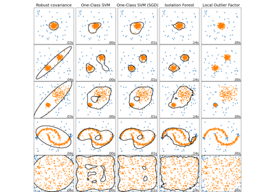
Comparing anomaly detection algorithms for outlier detection on toy datasets