1.5. Stochastic Gradient Descent#
Stochastic Gradient Descent (SGD) is a simple yet very efficient approach to fitting linear classifiers and regressors under convex loss functions such as (linear) Support Vector Machines and Logistic Regression. Even though SGD has been around in the machine learning community for a long time, it has received a considerable amount of attention just recently in the context of large-scale learning.
SGD has been successfully applied to large-scale and sparse machine learning problems often encountered in text classification and natural language processing. Given that the data is sparse, the classifiers in this module easily scale to problems with more than \(10^5\) training examples and more than \(10^5\) features.
Strictly speaking, SGD is merely an optimization technique and does not
correspond to a specific family of machine learning models. It is only a
way to train a model. Often, an instance of SGDClassifier or
SGDRegressor will have an equivalent estimator in
the scikit-learn API, potentially using a different optimization technique.
For example, using SGDClassifier(loss='log_loss') results in logistic regression,
i.e. a model equivalent to LogisticRegression
which is fitted via SGD instead of being fitted by one of the other solvers
in LogisticRegression. Similarly,
SGDRegressor(loss='squared_error', penalty='l2') and
Ridge solve the same optimization problem, via
different means.
The advantages of Stochastic Gradient Descent are:
Efficiency.
Ease of implementation (lots of opportunities for code tuning).
The disadvantages of Stochastic Gradient Descent include:
SGD requires a number of hyperparameters such as the regularization parameter and the number of iterations.
SGD is sensitive to feature scaling.
Warning
Make sure you permute (shuffle) your training data before fitting the model
or use shuffle=True to shuffle after each iteration (used by default).
Also, ideally, features should be standardized using e.g.
make_pipeline(StandardScaler(), SGDClassifier()) (see Pipelines).
1.5.1. Classification#
The class SGDClassifier implements a plain stochastic gradient
descent learning routine which supports different loss functions and
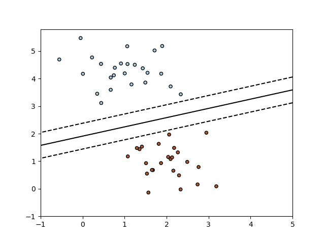
penalties for classification. Below is the decision boundary of a
SGDClassifier trained with the hinge loss, equivalent to a linear SVM.
As other classifiers, SGD has to be fitted with two arrays: an array X
of shape (n_samples, n_features) holding the training samples, and an
array y of shape (n_samples,) holding the target values (class labels)
for the training samples:
>>> from sklearn.linear_model import SGDClassifier
>>> X = [[0., 0.], [1., 1.]]
>>> y = [0, 1]
>>> clf = SGDClassifier(loss="hinge", penalty="l2", max_iter=5)
>>> clf.fit(X, y)
SGDClassifier(max_iter=5)
After being fitted, the model can then be used to predict new values:
>>> clf.predict([[2., 2.]])
array([1])
SGD fits a linear model to the training data. The coef_ attribute holds
the model parameters:
>>> clf.coef_
array([[9.9, 9.9]])
The intercept_ attribute holds the intercept (aka offset or bias):
>>> clf.intercept_
array([-9.9])
Whether or not the model should use an intercept, i.e. a biased
hyperplane, is controlled by the parameter fit_intercept.
The signed distance to the hyperplane (computed as the dot product between
the coefficients and the input sample, plus the intercept) is given by
SGDClassifier.decision_function:
>>> clf.decision_function([[2., 2.]])
array([29.6])
The concrete loss function can be set via the loss
parameter. SGDClassifier supports the following loss functions:
loss="hinge": (soft-margin) linear Support Vector Machine,loss="modified_huber": smoothed hinge loss,loss="log_loss": logistic regression,and all regression losses below. In this case the target is encoded as \(-1\) or \(1\), and the problem is treated as a regression problem. The predicted class then corresponds to the sign of the predicted target.
Please refer to the mathematical section below for formulas. The first two loss functions are lazy, they only update the model parameters if an example violates the margin constraint, which makes training very efficient and may result in sparser models (i.e. with more zero coefficients), even when \(L_2\) penalty is used.
Using loss="log_loss" or loss="modified_huber" enables the
predict_proba method, which gives a vector of probability estimates
\(P(y|x)\) per sample \(x\):
>>> clf = SGDClassifier(loss="log_loss", max_iter=5).fit(X, y)
>>> clf.predict_proba([[1., 1.]])
array([[0.00, 0.99]])
The concrete penalty can be set via the penalty parameter.
SGD supports the following penalties:
penalty="l2": \(L_2\) norm penalty oncoef_.penalty="l1": \(L_1\) norm penalty oncoef_.penalty="elasticnet": Convex combination of \(L_2\) and \(L_1\);(1 - l1_ratio) * L2 + l1_ratio * L1.
The default setting is penalty="l2". The \(L_1\) penalty leads to sparse
solutions, driving most coefficients to zero. The Elastic Net [11] solves
some deficiencies of the \(L_1\) penalty in the presence of highly correlated
attributes. The parameter l1_ratio controls the convex combination
of \(L_1\) and \(L_2\) penalty.
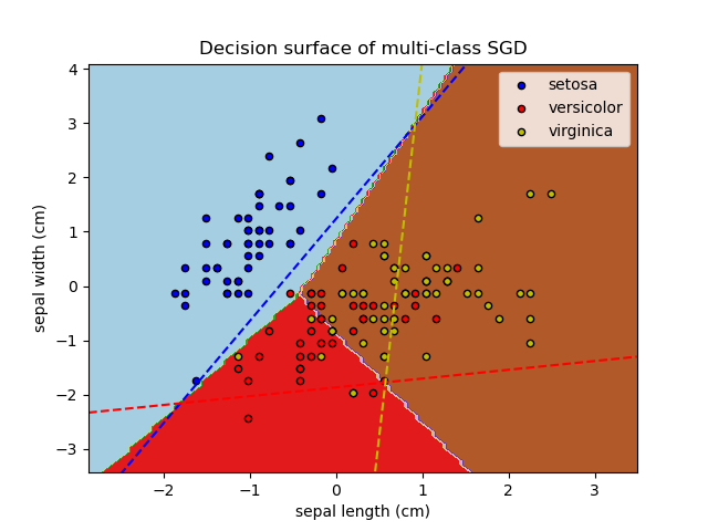
SGDClassifier supports multi-class classification by combining
multiple binary classifiers in a “one versus all” (OVA) scheme. For each
of the \(K\) classes, a binary classifier is learned that discriminates
between that and all other \(K-1\) classes. At testing time, we compute the
confidence score (i.e. the signed distances to the hyperplane) for each
classifier and choose the class with the highest confidence. The Figure
below illustrates the OVA approach on the iris dataset. The dashed
lines represent the three OVA classifiers; the background colors show
the decision surface induced by the three classifiers.
In the case of multi-class classification coef_ is a two-dimensional
array of shape (n_classes, n_features) and intercept_ is a
one-dimensional array of shape (n_classes,). The \(i\)-th row of coef_ holds
the weight vector of the OVA classifier for the \(i\)-th class; classes are
indexed in ascending order (see attribute classes_).
Note that, in principle, since they allow to create a probability model,
loss="log_loss" and loss="modified_huber" are more suitable for
one-vs-all classification.
SGDClassifier supports both weighted classes and weighted
instances via the fit parameters class_weight and sample_weight. See
the examples below and the docstring of SGDClassifier.fit for
further information.
SGDClassifier supports averaged SGD (ASGD) [10]. Averaging can be
enabled by setting average=True. ASGD performs the same updates as the
regular SGD (see Mathematical formulation), but instead of using
the last value of the coefficients as the coef_ attribute (i.e. the values
of the last update), coef_ is set instead to the average value of the
coefficients across all updates. The same is done for the intercept_
attribute. When using ASGD the learning rate can be larger and even constant,
leading on some datasets to a speed up in training time.
For classification with a logistic loss, another variant of SGD with an
averaging strategy is available with Stochastic Average Gradient (SAG)
algorithm, available as a solver in LogisticRegression.
Examples
1.5.2. Regression#
The class SGDRegressor implements a plain stochastic gradient
descent learning routine which supports different loss functions and
penalties to fit linear regression models. SGDRegressor is
well suited for regression problems with a large number of training
samples (> 10.000), for other problems we recommend Ridge,
Lasso, or ElasticNet.
The concrete loss function can be set via the loss
parameter. SGDRegressor supports the following loss functions:
loss="squared_error": Ordinary least squares,loss="huber": Huber loss for robust regression,loss="epsilon_insensitive": linear Support Vector Regression.
Please refer to the mathematical section below for formulas.
The Huber and epsilon-insensitive loss functions can be used for
robust regression. The width of the insensitive region has to be
specified via the parameter epsilon. This parameter depends on the
scale of the target variables.
The penalty parameter determines the regularization to be used (see
description above in the classification section).
SGDRegressor also supports averaged SGD [10] (here again, see
description above in the classification section).
For regression with a squared loss and a \(L_2\) penalty, another variant of
SGD with an averaging strategy is available with Stochastic Average
Gradient (SAG) algorithm, available as a solver in Ridge.
Examples
1.5.3. Online One-Class SVM#
The class sklearn.linear_model.SGDOneClassSVM implements an online
linear version of the One-Class SVM using a stochastic gradient descent.
Combined with kernel approximation techniques,
sklearn.linear_model.SGDOneClassSVM can be used to approximate the
solution of a kernelized One-Class SVM, implemented in
sklearn.svm.OneClassSVM, with a linear complexity in the number of
samples. Note that the complexity of a kernelized One-Class SVM is at best
quadratic in the number of samples.
sklearn.linear_model.SGDOneClassSVM is thus well suited for datasets
with a large number of training samples (over 10,000) for which the SGD
variant can be several orders of magnitude faster.
Mathematical details#
Its implementation is based on the implementation of the stochastic gradient descent. Indeed, the original optimization problem of the One-Class SVM is given by
where \(\nu \in (0, 1]\) is the user-specified parameter controlling the proportion of outliers and the proportion of support vectors. Getting rid of the slack variables \(\xi_i\) this problem is equivalent to
Multiplying by the constant \(\nu\) and introducing the intercept \(b = 1 - \rho\) we obtain the following equivalent optimization problem
This is similar to the optimization problems studied in section Mathematical formulation with \(y_i = 1, 1 \leq i \leq n\) and \(\alpha = \nu\), \(L\) being the hinge loss function and \(R\) being the \(L_2\) norm. We just need to add the term \(b\nu\) in the optimization loop.
As SGDClassifier and SGDRegressor, SGDOneClassSVM
supports averaged SGD. Averaging can be enabled by setting average=True.
Examples
1.5.4. Stochastic Gradient Descent for sparse data#
Note
The sparse implementation produces slightly different results from the dense implementation, due to a shrunk learning rate for the intercept. See Implementation details.
There is built-in support for sparse data given in any matrix in a format supported by scipy.sparse. For maximum efficiency, however, use the CSR matrix format as defined in scipy.sparse.csr_matrix.
Examples
1.5.5. Complexity#
The major advantage of SGD is its efficiency, which is basically linear in the number of training examples. If \(X\) is a matrix of size \(n \times p\) (with \(n\) samples and \(p\) features), training has a cost of \(O(k n \bar p)\), where \(k\) is the number of iterations (epochs) and \(\bar p\) is the average number of non-zero attributes per sample.
Recent theoretical results, however, show that the runtime to get some desired optimization accuracy does not increase as the training set size increases.
1.5.6. Stopping criterion#
The classes SGDClassifier and SGDRegressor provide two
criteria to stop the algorithm when a given level of convergence is reached:
With
early_stopping=True, the input data is split into a training set and a validation set. The model is then fitted on the training set, and the stopping criterion is based on the prediction score (using thescoremethod) computed on the validation set. The size of the validation set can be changed with the parametervalidation_fraction.With
early_stopping=False, the model is fitted on the entire input data and the stopping criterion is based on the objective function computed on the training data.
In both cases, the criterion is evaluated once by epoch, and the algorithm stops
when the criterion does not improve n_iter_no_change times in a row. The
improvement is evaluated with absolute tolerance tol, and the algorithm
stops in any case after a maximum number of iterations max_iter.
See Early stopping of Stochastic Gradient Descent for an example of the effects of early stopping.
1.5.7. Tips on Practical Use#
Stochastic Gradient Descent is sensitive to feature scaling, so it is highly recommended to scale your data. For example, scale each attribute on the input vector \(X\) to \([0,1]\) or \([-1,1]\), or standardize it to have mean \(0\) and variance \(1\). Note that the same scaling must be applied to the test vector to obtain meaningful results. This can be easily done using
StandardScaler:from sklearn.preprocessing import StandardScaler scaler = StandardScaler() scaler.fit(X_train) # Don't cheat - fit only on training data X_train = scaler.transform(X_train) X_test = scaler.transform(X_test) # apply same transformation to test data # Or better yet: use a pipeline! from sklearn.pipeline import make_pipeline est = make_pipeline(StandardScaler(), SGDClassifier()) est.fit(X_train) est.predict(X_test)
If your attributes have an intrinsic scale (e.g. word frequencies or indicator features) scaling is not needed.
Finding a reasonable regularization term \(\alpha\) is best done using automatic hyper-parameter search, e.g.
GridSearchCVorRandomizedSearchCV, usually in the range10.0**-np.arange(1,7).Empirically, we found that SGD converges after observing approximately \(10^6\) training samples. Thus, a reasonable first guess for the number of iterations is
max_iter = np.ceil(10**6 / n), wherenis the size of the training set.If you apply SGD to features extracted using PCA we found that it is often wise to scale the feature values by some constant
csuch that the average \(L_2\) norm of the training data equals one.We found that Averaged SGD works best with a larger number of features and a higher
eta0.
References
“Efficient BackProp” Y. LeCun, L. Bottou, G. Orr, K. Müller - In Neural Networks: Tricks of the Trade 1998.
1.5.8. Mathematical formulation#
We describe here the mathematical details of the SGD procedure. A good overview with convergence rates can be found in [12].
Given a set of training examples \(\{(x_1, y_1), \ldots, (x_n, y_n)\}\) where \(x_i \in \mathbf{R}^m\) and \(y_i \in \mathbf{R}\) (\(y_i \in \{-1, 1\}\) for classification), our goal is to learn a linear scoring function \(f(x) = w^T x + b\) with model parameters \(w \in \mathbf{R}^m\) and intercept \(b \in \mathbf{R}\). In order to make predictions for binary classification, we simply look at the sign of \(f(x)\). To find the model parameters, we minimize the regularized training error given by
where \(L\) is a loss function that measures model (mis)fit and \(R\) is a regularization term (aka penalty) that penalizes model complexity; \(\alpha > 0\) is a non-negative hyperparameter that controls the regularization strength.
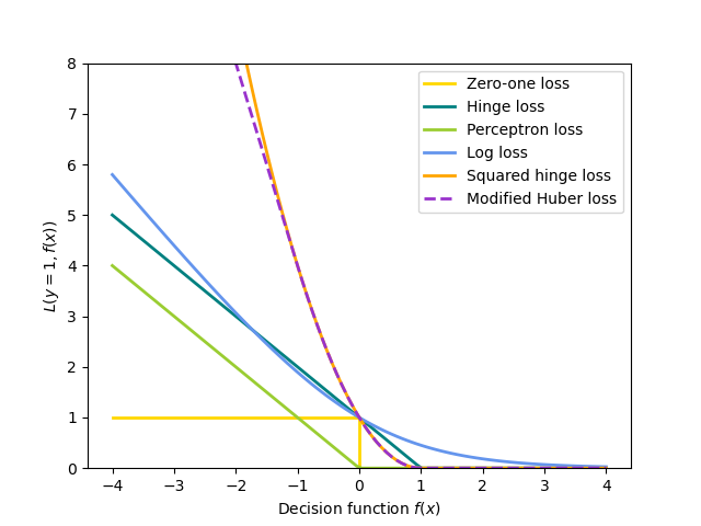
Loss functions details#
Different choices for \(L\) entail different classifiers or regressors:
Hinge (soft-margin): equivalent to Support Vector Classification. \(L(y_i, f(x_i)) = \max(0, 1 - y_i f(x_i))\).
Perceptron: \(L(y_i, f(x_i)) = \max(0, - y_i f(x_i))\).
Modified Huber: \(L(y_i, f(x_i)) = \max(0, 1 - y_i f(x_i))^2\) if \(y_i f(x_i) > -1\), and \(L(y_i, f(x_i)) = -4 y_i f(x_i)\) otherwise.
Log Loss: equivalent to Logistic Regression. \(L(y_i, f(x_i)) = \log(1 + \exp (-y_i f(x_i)))\).
Squared Error: Linear regression (Ridge or Lasso depending on \(R\)). \(L(y_i, f(x_i)) = \frac{1}{2}(y_i - f(x_i))^2\).
Huber: less sensitive to outliers than least-squares. It is equivalent to least squares when \(|y_i - f(x_i)| \leq \varepsilon\), and \(L(y_i, f(x_i)) = \varepsilon |y_i - f(x_i)| - \frac{1}{2} \varepsilon^2\) otherwise.
Epsilon-Insensitive: (soft-margin) equivalent to Support Vector Regression. \(L(y_i, f(x_i)) = \max(0, |y_i - f(x_i)| - \varepsilon)\).
All of the above loss functions can be regarded as an upper bound on the misclassification error (Zero-one loss) as shown in the Figure below.
Popular choices for the regularization term \(R\) (the penalty
parameter) include:
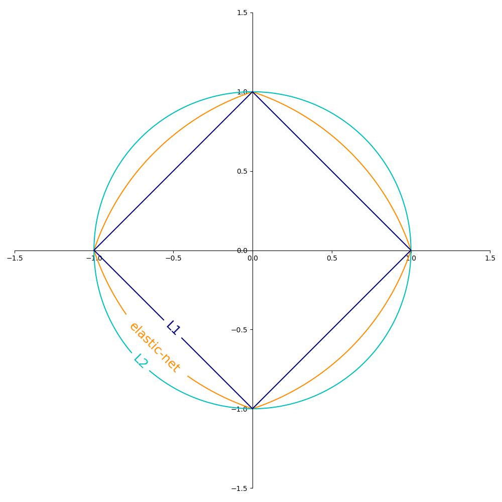
\(L_2\) norm: \(R(w) := \frac{1}{2} \sum_{j=1}^{m} w_j^2 = \frac{1}{2} ||w||_2^2\),
\(L_1\) norm: \(R(w) := \sum_{j=1}^{m} |w_j|\), which leads to sparse solutions.
Elastic Net: \(R(w) := \frac{\rho}{2} \sum_{j=1}^{n} w_j^2 + (1-\rho) \sum_{j=1}^{m} |w_j|\), a convex combination of \(L_2\) and \(L_1\), where \(\rho\) is given by
1 - l1_ratio.
The Figure below shows the contours of the different regularization terms in a 2-dimensional parameter space (\(m=2\)) when \(R(w) = 1\).
1.5.8.1. SGD#
Stochastic gradient descent is an optimization method for unconstrained optimization problems. In contrast to (batch) gradient descent, SGD approximates the true gradient of \(E(w,b)\) by considering a single training example at a time.
The class SGDClassifier implements a first-order SGD learning
routine. The algorithm iterates over the training examples and for each
example updates the model parameters according to the update rule given by
where \(\eta\) is the learning rate which controls the step-size in the parameter space. The intercept \(b\) is updated similarly but without regularization (and with additional decay for sparse matrices, as detailed in Implementation details).
The learning rate \(\eta\) can be either constant or gradually decaying. For
classification, the default learning rate schedule (learning_rate='optimal')
is given by
where \(t\) is the time step (there are a total of n_samples * n_iter
time steps), \(t_0\) is determined based on a heuristic proposed by Léon Bottou
such that the expected initial updates are comparable with the expected
size of the weights (this assumes that the norm of the training samples is
approximately 1). The exact definition can be found in _init_t in BaseSGD.
For regression the default learning rate schedule is inverse scaling
(learning_rate='invscaling'), given by
where \(\eta_0\) and \(power\_t\) are hyperparameters chosen by the
user via eta0 and power_t, respectively.
For a constant learning rate use learning_rate='constant' and use eta0
to specify the learning rate.
For an adaptively decreasing learning rate, use learning_rate='adaptive'
and use eta0 to specify the starting learning rate. When the stopping
criterion is reached, the learning rate is divided by 5, and the algorithm
does not stop. The algorithm stops when the learning rate goes below 1e-6.
The model parameters can be accessed through the coef_ and
intercept_ attributes: coef_ holds the weights \(w\) and
intercept_ holds \(b\).
When using Averaged SGD (with the average parameter), coef_ is set to the
average weight across all updates:
coef_ \(= \frac{1}{T} \sum_{t=0}^{T-1} w^{(t)}\),
where \(T\) is the total number of updates, found in the t_ attribute.
1.5.9. Implementation details#
The implementation of SGD is influenced by the Stochastic Gradient SVM of
[7].
Similar to SvmSGD,
the weight vector is represented as the product of a scalar and a vector
which allows an efficient weight update in the case of \(L_2\) regularization.
In the case of sparse input X, the intercept is updated with a
smaller learning rate (multiplied by 0.01) to account for the fact that
it is updated more frequently. Training examples are picked up sequentially
and the learning rate is lowered after each observed example. We adopted the
learning rate schedule from [8].
For multi-class classification, a “one versus all” approach is used.
We use the truncated gradient algorithm proposed in [9]
for \(L_1\) regularization (and the Elastic Net).
The code is written in Cython.
References
