2.1. Gaussian mixture models#
sklearn.mixture is a package which enables one to learn
Gaussian Mixture Models (diagonal, spherical, tied and full covariance
matrices supported), sample them, and estimate them from
data. Facilities to help determine the appropriate number of
components are also provided.
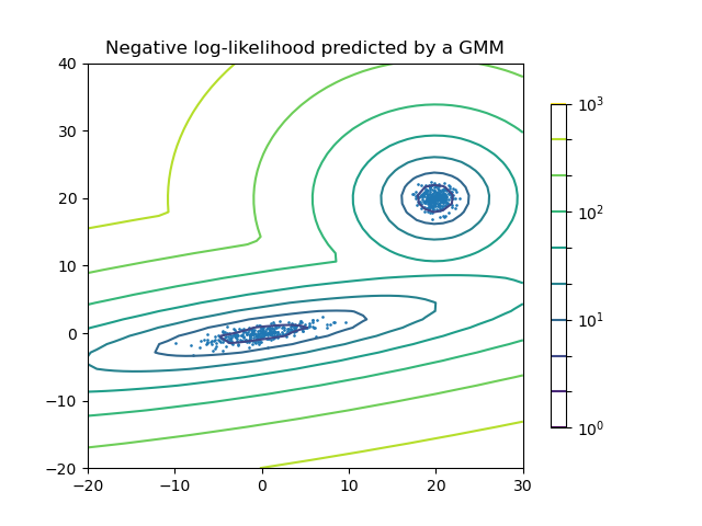
Two-component Gaussian mixture model: data points, and equi-probability surfaces of the model.#
A Gaussian mixture model is a probabilistic model that assumes all the data points are generated from a mixture of a finite number of Gaussian distributions with unknown parameters. One can think of mixture models as generalizing k-means clustering to incorporate information about the covariance structure of the data as well as the centers of the latent Gaussians.
Scikit-learn implements different classes to estimate Gaussian mixture models, that correspond to different estimation strategies, detailed below.
2.1.1. Gaussian Mixture#
The GaussianMixture object implements the
expectation-maximization (EM)
algorithm for fitting mixture-of-Gaussian models. It can also draw
confidence ellipsoids for multivariate models, and compute the
Bayesian Information Criterion to assess the number of clusters in the
data. A GaussianMixture.fit method is provided that learns a Gaussian
Mixture Model from training data. Given test data, it can assign to each
sample the Gaussian it most probably belongs to using
the GaussianMixture.predict method.
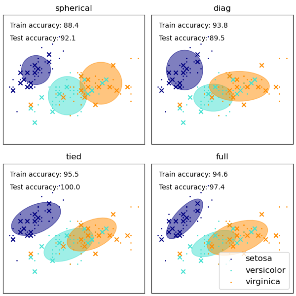
The GaussianMixture comes with different options to constrain the
covariance of the difference classes estimated: spherical, diagonal, tied or
full covariance.
Examples
See GMM covariances for an example of using the Gaussian mixture as clustering on the iris dataset.
See Density Estimation for a Gaussian mixture for an example on plotting the density estimation.
Pros and cons of class GaussianMixture#
Pros
- Speed:
It is the fastest algorithm for learning mixture models
- Agnostic:
As this algorithm maximizes only the likelihood, it will not bias the means towards zero, or bias the cluster sizes to have specific structures that might or might not apply.
Cons
- Singularities:
When one has insufficiently many points per mixture, estimating the covariance matrices becomes difficult, and the algorithm is known to diverge and find solutions with infinite likelihood unless one regularizes the covariances artificially.
- Number of components:
This algorithm will always use all the components it has access to, needing held-out data or information theoretical criteria to decide how many components to use in the absence of external cues.
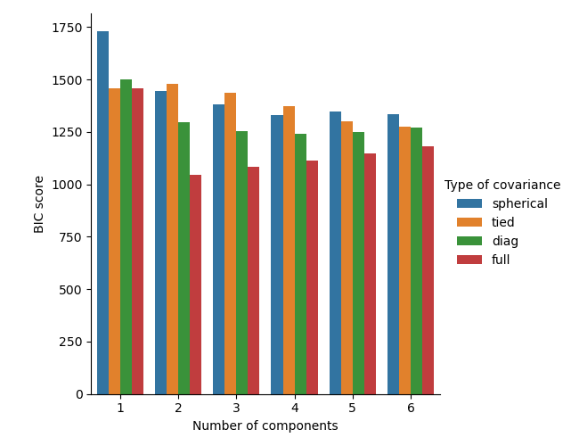
Selecting the number of components in a classical Gaussian Mixture model#
The BIC criterion can be used to select the number of components in a Gaussian Mixture in an efficient way. In theory, it recovers the true number of components only in the asymptotic regime (i.e. if much data is available and assuming that the data was actually generated i.i.d. from a mixture of Gaussian distributions). Note that using a Variational Bayesian Gaussian mixture avoids the specification of the number of components for a Gaussian mixture model.
Examples
See Gaussian Mixture Model Selection for an example of model selection performed with classical Gaussian mixture.
Estimation algorithm expectation-maximization#
The main difficulty in learning Gaussian mixture models from unlabeled data is that one usually doesn’t know which points came from which latent component (if one has access to this information it gets very easy to fit a separate Gaussian distribution to each set of points). Expectation-maximization is a well-founded statistical algorithm to get around this problem by an iterative process. First one assumes random components (randomly centered on data points, learned from k-means, or even just normally distributed around the origin) and computes for each point a probability of being generated by each component of the model. Then, one tweaks the parameters to maximize the likelihood of the data given those assignments. Repeating this process is guaranteed to always converge to a local optimum.
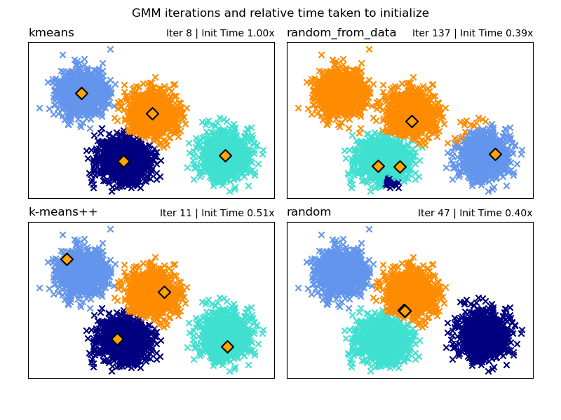
Choice of the Initialization method#
There is a choice of four initialization methods (as well as inputting user defined initial means) to generate the initial centers for the model components:
- k-means (default)
This applies a traditional k-means clustering algorithm. This can be computationally expensive compared to other initialization methods.
- k-means++
This uses the initialization method of k-means clustering: k-means++. This will pick the first center at random from the data. Subsequent centers will be chosen from a weighted distribution of the data favouring points further away from existing centers. k-means++ is the default initialization for k-means so will be quicker than running a full k-means but can still take a significant amount of time for large data sets with many components.
- random_from_data
This will pick random data points from the input data as the initial centers. This is a very fast method of initialization but can produce non-convergent results if the chosen points are too close to each other.
- random
Centers are chosen as a small perturbation away from the mean of all data. This method is simple but can lead to the model taking longer to converge.
Examples
See GMM Initialization Methods for an example of using different initializations in Gaussian Mixture.
2.1.2. Variational Bayesian Gaussian Mixture#
The BayesianGaussianMixture object implements a variant of the
Gaussian mixture model with variational inference algorithms. The API is
similar to the one defined by GaussianMixture.
Estimation algorithm: variational inference
Variational inference is an extension of expectation-maximization that maximizes a lower bound on model evidence (including priors) instead of data likelihood. The principle behind variational methods is the same as expectation-maximization (that is both are iterative algorithms that alternate between finding the probabilities for each point to be generated by each mixture and fitting the mixture to these assigned points), but variational methods add regularization by integrating information from prior distributions. This avoids the singularities often found in expectation-maximization solutions but introduces some subtle biases to the model. Inference is often notably slower, but not usually as much so as to render usage unpractical.
Due to its Bayesian nature, the variational algorithm needs more hyperparameters
than expectation-maximization, the most important of these being the
concentration parameter weight_concentration_prior. Specifying a low value
for the concentration prior will make the model put most of the weight on a few
components and set the remaining components’ weights very close to zero. High
values of the concentration prior will allow a larger number of components to
be active in the mixture.
The parameters implementation of the BayesianGaussianMixture class
proposes two types of prior for the weights distribution: a finite mixture model
with Dirichlet distribution and an infinite mixture model with the Dirichlet
Process. In practice Dirichlet Process inference algorithm is approximated and
uses a truncated distribution with a fixed maximum number of components (called
the Stick-breaking representation). The number of components actually used
almost always depends on the data.
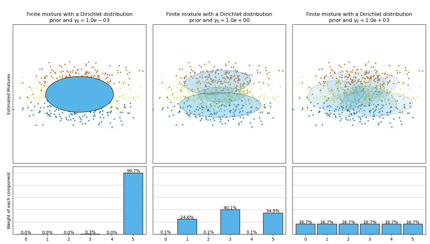
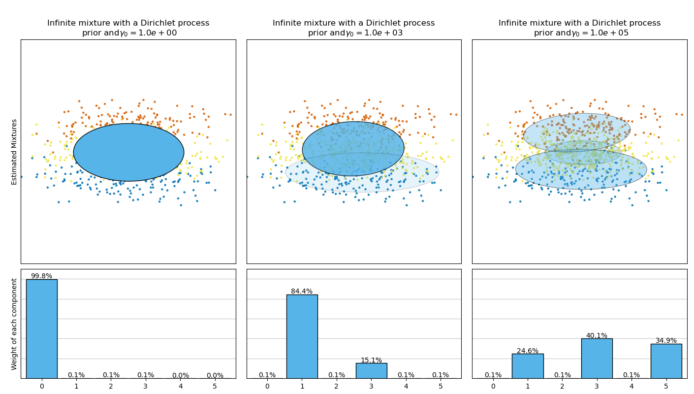
The next figure compares the results obtained for the different types of the
weight concentration prior (parameter weight_concentration_prior_type)
for different values of weight_concentration_prior.
Here, we can see the value of the weight_concentration_prior parameter
has a strong impact on the effective number of active components obtained. We
can also notice that large values for the concentration weight prior lead to
more uniform weights when the type of prior is ‘dirichlet_distribution’ while
this is not necessarily the case for the ‘dirichlet_process’ type (used by
default).
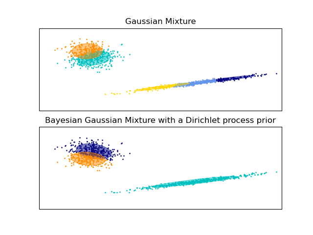
The examples below compare Gaussian mixture models with a fixed number of
components, to the variational Gaussian mixture models with a Dirichlet process
prior. Here, a classical Gaussian mixture is fitted with 5 components on a
dataset composed of 2 clusters. We can see that the variational Gaussian mixture
with a Dirichlet process prior is able to limit itself to only 2 components
whereas the Gaussian mixture fits the data with a fixed number of components
that has to be set a priori by the user. In this case the user has selected
n_components=5 which does not match the true generative distribution of this
toy dataset. Note that with very little observations, the variational Gaussian
mixture models with a Dirichlet process prior can take a conservative stand, and
fit only one component.
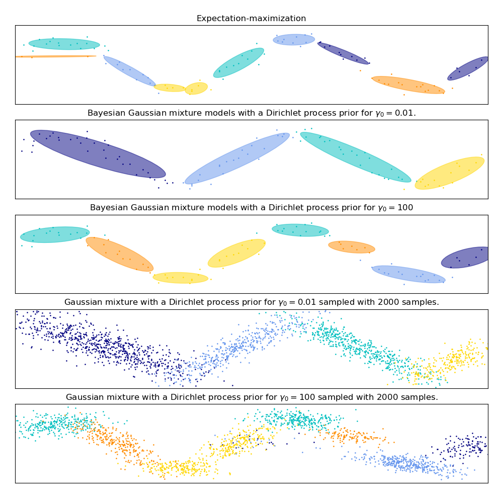
On the following figure we are fitting a dataset not well-depicted by a
Gaussian mixture. Adjusting the weight_concentration_prior, parameter of the
BayesianGaussianMixture controls the number of components used to fit
this data. We also present on the last two plots a random sampling generated
from the two resulting mixtures.
Examples
See Gaussian Mixture Model Ellipsoids for an example on plotting the confidence ellipsoids for both
GaussianMixtureandBayesianGaussianMixture.Gaussian Mixture Model Sine Curve shows using
GaussianMixtureandBayesianGaussianMixtureto fit a sine wave.See Concentration Prior Type Analysis of Variation Bayesian Gaussian Mixture for an example plotting the confidence ellipsoids for the
BayesianGaussianMixturewith differentweight_concentration_prior_typefor different values of the parameterweight_concentration_prior.
Pros and cons of variational inference with BayesianGaussianMixture#
Pros
- Automatic selection:
When
weight_concentration_prioris small enough andn_componentsis larger than what is found necessary by the model, the Variational Bayesian mixture model has a natural tendency to set some mixture weights values close to zero. This makes it possible to let the model choose a suitable number of effective components automatically. Only an upper bound of this number needs to be provided. Note however that the “ideal” number of active components is very application specific and is typically ill-defined in a data exploration setting.- Less sensitivity to the number of parameters:
Unlike finite models, which will almost always use all components as much as they can, and hence will produce wildly different solutions for different numbers of components, the variational inference with a Dirichlet process prior (
weight_concentration_prior_type='dirichlet_process') won’t change much with changes to the parameters, leading to more stability and less tuning.- Regularization:
Due to the incorporation of prior information, variational solutions have less pathological special cases than expectation-maximization solutions.
Cons
- Speed:
The extra parametrization necessary for variational inference makes inference slower, although not by much.
- Hyperparameters:
This algorithm needs an extra hyperparameter that might need experimental tuning via cross-validation.
- Bias:
There are many implicit biases in the inference algorithms (and also in the Dirichlet process if used), and whenever there is a mismatch between these biases and the data it might be possible to fit better models using a finite mixture.
2.1.2.1. The Dirichlet Process#
Here we describe variational inference algorithms on Dirichlet process mixture. The Dirichlet process is a prior probability distribution on clusterings with an infinite, unbounded, number of partitions. Variational techniques let us incorporate this prior structure on Gaussian mixture models at almost no penalty in inference time, comparing with a finite Gaussian mixture model.
An important question is how can the Dirichlet process use an infinite, unbounded number of clusters and still be consistent. While a full explanation doesn’t fit this manual, one can think of its stick breaking process analogy to help understanding it. The stick breaking process is a generative story for the Dirichlet process. We start with a unit-length stick and in each step we break off a portion of the remaining stick. Each time, we associate the length of the piece of the stick to the proportion of points that falls into a group of the mixture. At the end, to represent the infinite mixture, we associate the last remaining piece of the stick to the proportion of points that don’t fall into all the other groups. The length of each piece is a random variable with probability proportional to the concentration parameter. Smaller values of the concentration will divide the unit-length into larger pieces of the stick (defining more concentrated distribution). Larger concentration values will create smaller pieces of the stick (increasing the number of components with non zero weights).
Variational inference techniques for the Dirichlet process still work with a finite approximation to this infinite mixture model, but instead of having to specify a priori how many components one wants to use, one just specifies the concentration parameter and an upper bound on the number of mixture components (this upper bound, assuming it is higher than the “true” number of components, affects only algorithmic complexity, not the actual number of components used).
