Note
Go to the end to download the full example code or to run this example in your browser via JupyterLite or Binder.
Pipelining: chaining a PCA and a logistic regression#
The PCA does an unsupervised dimensionality reduction, while the logistic regression does the prediction.
We use a GridSearchCV to set the dimensionality of the PCA
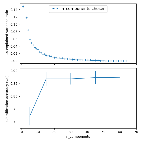
Best parameter (CV score=0.874):
{'logistic__C': np.float64(21.54434690031882), 'pca__n_components': 60}
# Authors: The scikit-learn developers
# SPDX-License-Identifier: BSD-3-Clause

import matplotlib.pyplot as plt
import numpy as np
import polars as pl

from sklearn import datasets
from sklearn.decomposition import PCA
from sklearn.linear_model import LogisticRegression
from sklearn.model_selection import GridSearchCV
from sklearn.pipeline import Pipeline
from sklearn.preprocessing import StandardScaler

# Define a pipeline to search for the best combination of PCA truncation
# and classifier regularization.
pca = PCA()
# Define a Standard Scaler to normalize inputs
scaler = StandardScaler()

# set the tolerance to a large value to make the example faster
logistic = LogisticRegression(max_iter=10000, tol=0.1)
pipe = Pipeline(steps=[("scaler", scaler), ("pca", pca), ("logistic", logistic)])

X_digits, y_digits = datasets.load_digits(return_X_y=True)
# Parameters of pipelines can be set using '__' separated parameter names:
param_grid = {
    "pca__n_components": [5, 15, 30, 45, 60],
    "logistic__C": np.logspace(-4, 4, 4),
}
search = GridSearchCV(pipe, param_grid, n_jobs=2)
search.fit(X_digits, y_digits)
print("Best parameter (CV score=%0.3f):" % search.best_score_)
print(search.best_params_)

# Plot the PCA spectrum
pca.fit(X_digits)

fig, (ax0, ax1) = plt.subplots(nrows=2, sharex=True, figsize=(6, 6))
ax0.plot(
    np.arange(1, pca.n_components_ + 1), pca.explained_variance_ratio_, "+", linewidth=2
)
ax0.set_ylabel("PCA explained variance ratio")

ax0.axvline(
    search.best_estimator_.named_steps["pca"].n_components,
    linestyle=":",
    label="n_components chosen",
)
ax0.legend(prop=dict(size=12))

# For each number of components, find the best classifier results
components_col = "param_pca__n_components"
is_max_test_score = pl.col("mean_test_score") == pl.col("mean_test_score").max()
best_clfs = (
    pl.LazyFrame(search.cv_results_)
    .filter(is_max_test_score.over(components_col))
    .unique(components_col)
    .sort(components_col)
    .collect()
)
ax1.errorbar(
    best_clfs[components_col],
    best_clfs["mean_test_score"],
    yerr=best_clfs["std_test_score"],
)
ax1.set_ylabel("Classification accuracy (val)")
ax1.set_xlabel("n_components")

plt.xlim(-1, 70)

plt.tight_layout()
plt.show()
Total running time of the script: (0 minutes 0.883 seconds)
Related examples
Effect of transforming the targets in regression model
Effect of transforming the targets in regression model
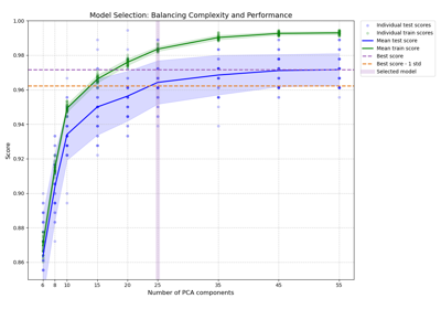
Balance model complexity and cross-validated score
Balance model complexity and cross-validated score

Comparing randomized search and grid search for hyperparameter estimation
Comparing randomized search and grid search for hyperparameter estimation
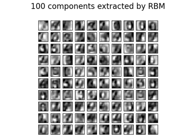
Restricted Boltzmann Machine features for digit classification
Restricted Boltzmann Machine features for digit classification