Note
Go to the end to download the full example code or to run this example in your browser via JupyterLite or Binder.
Demo of DBSCAN clustering algorithm#
DBSCAN (Density-Based Spatial Clustering of Applications with Noise) finds core samples in regions of high density and expands clusters from them. This algorithm is good for data which contains clusters of similar density.
See the Comparing different clustering algorithms on toy datasets example for a demo of different clustering algorithms on 2D datasets.
# Authors: The scikit-learn developers
# SPDX-License-Identifier: BSD-3-Clause
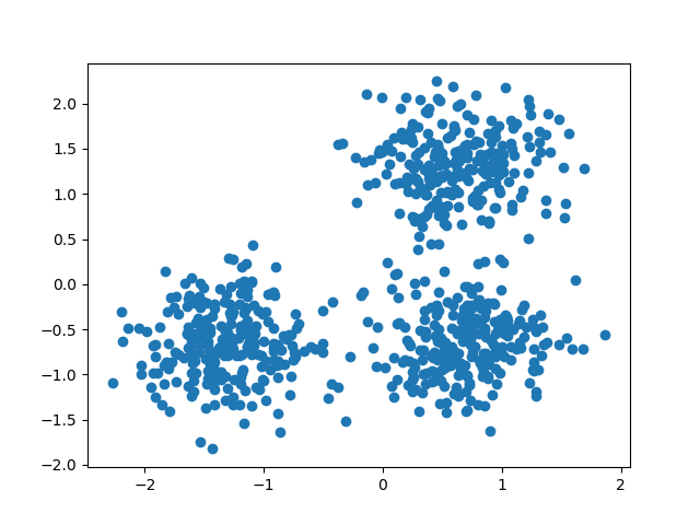
Data generation#
We use make_blobs to create 3 synthetic clusters.
from sklearn.datasets import make_blobs
from sklearn.preprocessing import StandardScaler

centers = [[1, 1], [-1, -1], [1, -1]]
X, labels_true = make_blobs(
    n_samples=750, centers=centers, cluster_std=0.4, random_state=0
)

X = StandardScaler().fit_transform(X)
We can visualize the resulting data:
import matplotlib.pyplot as plt

plt.scatter(X[:, 0], X[:, 1])
plt.show()
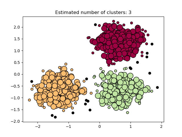
Compute DBSCAN#
One can access the labels assigned by DBSCAN using
the labels_ attribute. Noisy samples are given the label \(-1\).
import numpy as np
from sklearn import metrics
from sklearn.cluster import DBSCAN
db = DBSCAN(eps=0.3, min_samples=10).fit(X)
labels = db.labels_
# Number of clusters in labels, ignoring noise if present.
n_clusters_ = len(set(labels)) - (1 if -1 in labels else 0)
n_noise_ = list(labels).count(-1)
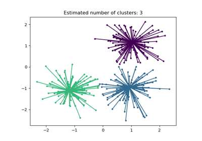
print("Estimated number of clusters: %d" % n_clusters_)
print("Estimated number of noise points: %d" % n_noise_)
Estimated number of clusters: 3
Estimated number of noise points: 18
Clustering algorithms are fundamentally unsupervised learning methods.
However, since make_blobs gives access to the true
labels of the synthetic clusters, it is possible to use evaluation metrics
that leverage this “supervised” ground truth information to quantify the
quality of the resulting clusters. Examples of such metrics are the
homogeneity, completeness, V-measure, Rand-Index, Adjusted Rand-Index and
Adjusted Mutual Information (AMI).
If the ground truth labels are not known, evaluation can only be performed using the model results itself. In that case, the Silhouette Coefficient comes in handy.
For more information, see the Adjustment for chance in clustering performance evaluation example or the Clustering performance evaluation module.
print(f"Homogeneity: {metrics.homogeneity_score(labels_true, labels):.3f}")
print(f"Completeness: {metrics.completeness_score(labels_true, labels):.3f}")
print(f"V-measure: {metrics.v_measure_score(labels_true, labels):.3f}")
print(f"Adjusted Rand Index: {metrics.adjusted_rand_score(labels_true, labels):.3f}")
print(
    "Adjusted Mutual Information:"
    f" {metrics.adjusted_mutual_info_score(labels_true, labels):.3f}"
)
print(f"Silhouette Coefficient: {metrics.silhouette_score(X, labels):.3f}")
Homogeneity: 0.953
Completeness: 0.883
V-measure: 0.917
Adjusted Rand Index: 0.952
Adjusted Mutual Information: 0.916
Silhouette Coefficient: 0.626
Plot results#
Core samples (large dots) and non-core samples (small dots) are color-coded according to the assigned cluster. Samples tagged as noise are represented in black.
unique_labels = set(labels)
core_samples_mask = np.zeros_like(labels, dtype=bool)
core_samples_mask[db.core_sample_indices_] = True

colors = [plt.cm.Spectral(each) for each in np.linspace(0, 1, len(unique_labels))]
for k, col in zip(unique_labels, colors):
    if k == -1:
        # Black used for noise.
        col = [0, 0, 0, 1]

    class_member_mask = labels == k

    xy = X[class_member_mask & core_samples_mask]
    plt.plot(
        xy[:, 0],
        xy[:, 1],
        "o",
        markerfacecolor=tuple(col),
        markeredgecolor="k",
        markersize=14,
    )

    xy = X[class_member_mask & ~core_samples_mask]
    plt.plot(
        xy[:, 0],
        xy[:, 1],
        "o",
        markerfacecolor=tuple(col),
        markeredgecolor="k",
        markersize=6,
    )

plt.title(f"Estimated number of clusters: {n_clusters_}")
plt.show()
Total running time of the script: (0 minutes 0.107 seconds)
Related examples
Adjustment for chance in clustering performance evaluation