LogisticRegression#
- class sklearn.linear_model.LogisticRegression(penalty='l2', *, dual=False, tol=0.0001, C=1.0, fit_intercept=True, intercept_scaling=1, class_weight=None, random_state=None, solver='lbfgs', max_iter=100, multi_class='deprecated', verbose=0, warm_start=False, n_jobs=None, l1_ratio=None)[source]#
Logistic Regression (aka logit, MaxEnt) classifier.
This class implements regularized logistic regression using the ‘liblinear’ library, ‘newton-cg’, ‘sag’, ‘saga’ and ‘lbfgs’ solvers. Note that regularization is applied by default. It can handle both dense and sparse input. Use C-ordered arrays or CSR matrices containing 64-bit floats for optimal performance; any other input format will be converted (and copied).
The ‘newton-cg’, ‘sag’, and ‘lbfgs’ solvers support only L2 regularization with primal formulation, or no regularization. The ‘liblinear’ solver supports both L1 and L2 regularization, with a dual formulation only for the L2 penalty. The Elastic-Net regularization is only supported by the ‘saga’ solver.
For multiclass problems, only ‘newton-cg’, ‘sag’, ‘saga’ and ‘lbfgs’ handle multinomial loss. ‘liblinear’ and ‘newton-cholesky’ only handle binary classification but can be extended to handle multiclass by using
OneVsRestClassifier.Read more in the User Guide.
- Parameters:
- penalty{‘l1’, ‘l2’, ‘elasticnet’, None}, default=’l2’
Specify the norm of the penalty:
None: no penalty is added;'l2': add a L2 penalty term and it is the default choice;'l1': add a L1 penalty term;'elasticnet': both L1 and L2 penalty terms are added.
Warning
Some penalties may not work with some solvers. See the parameter
solverbelow, to know the compatibility between the penalty and solver.Added in version 0.19: l1 penalty with SAGA solver (allowing ‘multinomial’ + L1)
- dualbool, default=False
Dual (constrained) or primal (regularized, see also this equation) formulation. Dual formulation is only implemented for l2 penalty with liblinear solver. Prefer dual=False when n_samples > n_features.
- tolfloat, default=1e-4
Tolerance for stopping criteria.
- Cfloat, default=1.0
Inverse of regularization strength; must be a positive float. Like in support vector machines, smaller values specify stronger regularization.
- fit_interceptbool, default=True
Specifies if a constant (a.k.a. bias or intercept) should be added to the decision function.
- intercept_scalingfloat, default=1
Useful only when the solver ‘liblinear’ is used and self.fit_intercept is set to True. In this case, x becomes [x, self.intercept_scaling], i.e. a “synthetic” feature with constant value equal to intercept_scaling is appended to the instance vector. The intercept becomes
intercept_scaling * synthetic_feature_weight.Note! the synthetic feature weight is subject to l1/l2 regularization as all other features. To lessen the effect of regularization on synthetic feature weight (and therefore on the intercept) intercept_scaling has to be increased.
- class_weightdict or ‘balanced’, default=None
Weights associated with classes in the form
{class_label: weight}. If not given, all classes are supposed to have weight one.The “balanced” mode uses the values of y to automatically adjust weights inversely proportional to class frequencies in the input data as
n_samples / (n_classes * np.bincount(y)).Note that these weights will be multiplied with sample_weight (passed through the fit method) if sample_weight is specified.
Added in version 0.17: class_weight=’balanced’
- random_stateint, RandomState instance, default=None
Used when
solver== ‘sag’, ‘saga’ or ‘liblinear’ to shuffle the data. See Glossary for details.- solver{‘lbfgs’, ‘liblinear’, ‘newton-cg’, ‘newton-cholesky’, ‘sag’, ‘saga’}, default=’lbfgs’
Algorithm to use in the optimization problem. Default is ‘lbfgs’. To choose a solver, you might want to consider the following aspects:
For small datasets, ‘liblinear’ is a good choice, whereas ‘sag’ and ‘saga’ are faster for large ones;
For multiclass problems, all solvers except ‘liblinear’ minimize the full multinomial loss;
‘liblinear’ can only handle binary classification by default. To apply a one-versus-rest scheme for the multiclass setting one can wrap it with the
OneVsRestClassifier.‘newton-cholesky’ is a good choice for
n_samples>>n_features * n_classes, especially with one-hot encoded categorical features with rare categories. Be aware that the memory usage of this solver has a quadratic dependency onn_features * n_classesbecause it explicitly computes the full Hessian matrix.
Warning
The choice of the algorithm depends on the penalty chosen and on (multinomial) multiclass support:
solver
penalty
multinomial multiclass
‘lbfgs’
‘l2’, None
yes
‘liblinear’
‘l1’, ‘l2’
no
‘newton-cg’
‘l2’, None
yes
‘newton-cholesky’
‘l2’, None
no
‘sag’
‘l2’, None
yes
‘saga’
‘elasticnet’, ‘l1’, ‘l2’, None
yes
Note
‘sag’ and ‘saga’ fast convergence is only guaranteed on features with approximately the same scale. You can preprocess the data with a scaler from
sklearn.preprocessing.See also
Refer to the User Guide for more information regarding
LogisticRegressionand more specifically the Table summarizing solver/penalty supports.Added in version 0.17: Stochastic Average Gradient descent solver.
Added in version 0.19: SAGA solver.
Changed in version 0.22: The default solver changed from ‘liblinear’ to ‘lbfgs’ in 0.22.
Added in version 1.2: newton-cholesky solver.
- max_iterint, default=100
Maximum number of iterations taken for the solvers to converge.
- multi_class{‘auto’, ‘ovr’, ‘multinomial’}, default=’auto’
If the option chosen is ‘ovr’, then a binary problem is fit for each label. For ‘multinomial’ the loss minimised is the multinomial loss fit across the entire probability distribution, even when the data is binary. ‘multinomial’ is unavailable when solver=’liblinear’. ‘auto’ selects ‘ovr’ if the data is binary, or if solver=’liblinear’, and otherwise selects ‘multinomial’.
Added in version 0.18: Stochastic Average Gradient descent solver for ‘multinomial’ case.
Changed in version 0.22: Default changed from ‘ovr’ to ‘auto’ in 0.22.
Deprecated since version 1.5:
multi_classwas deprecated in version 1.5 and will be removed in 1.7. From then on, the recommended ‘multinomial’ will always be used forn_classes >= 3. Solvers that do not support ‘multinomial’ will raise an error. Usesklearn.multiclass.OneVsRestClassifier(LogisticRegression())if you still want to use OvR.- verboseint, default=0
For the liblinear and lbfgs solvers set verbose to any positive number for verbosity.
- warm_startbool, default=False
When set to True, reuse the solution of the previous call to fit as initialization, otherwise, just erase the previous solution. Useless for liblinear solver. See the Glossary.
Added in version 0.17: warm_start to support lbfgs, newton-cg, sag, saga solvers.
- n_jobsint, default=None
Number of CPU cores used when parallelizing over classes if multi_class=’ovr’”. This parameter is ignored when the
solveris set to ‘liblinear’ regardless of whether ‘multi_class’ is specified or not.Nonemeans 1 unless in ajoblib.parallel_backendcontext.-1means using all processors. See Glossary for more details.- l1_ratiofloat, default=None
The Elastic-Net mixing parameter, with
0 <= l1_ratio <= 1. Only used ifpenalty='elasticnet'. Settingl1_ratio=0is equivalent to usingpenalty='l2', while settingl1_ratio=1is equivalent to usingpenalty='l1'. For0 < l1_ratio <1, the penalty is a combination of L1 and L2.
- Attributes:
- classes_ndarray of shape (n_classes, )
A list of class labels known to the classifier.
- coef_ndarray of shape (1, n_features) or (n_classes, n_features)
Coefficient of the features in the decision function.
coef_is of shape (1, n_features) when the given problem is binary. In particular, whenmulti_class='multinomial',coef_corresponds to outcome 1 (True) and-coef_corresponds to outcome 0 (False).- intercept_ndarray of shape (1,) or (n_classes,)
Intercept (a.k.a. bias) added to the decision function.
If
fit_interceptis set to False, the intercept is set to zero.intercept_is of shape (1,) when the given problem is binary. In particular, whenmulti_class='multinomial',intercept_corresponds to outcome 1 (True) and-intercept_corresponds to outcome 0 (False).- n_features_in_int
Number of features seen during fit.
Added in version 0.24.
- feature_names_in_ndarray of shape (
n_features_in_,) Names of features seen during fit. Defined only when
Xhas feature names that are all strings.Added in version 1.0.
- n_iter_ndarray of shape (n_classes,) or (1, )
Actual number of iterations for all classes. If binary or multinomial, it returns only 1 element. For liblinear solver, only the maximum number of iteration across all classes is given.
Changed in version 0.20: In SciPy <= 1.0.0 the number of lbfgs iterations may exceed
max_iter.n_iter_will now report at mostmax_iter.
See also
SGDClassifierIncrementally trained logistic regression (when given the parameter
loss="log_loss").LogisticRegressionCVLogistic regression with built-in cross validation.
Notes
The underlying C implementation uses a random number generator to select features when fitting the model. It is thus not uncommon, to have slightly different results for the same input data. If that happens, try with a smaller tol parameter.
Predict output may not match that of standalone liblinear in certain cases. See differences from liblinear in the narrative documentation.
References
- L-BFGS-B – Software for Large-scale Bound-constrained Optimization
Ciyou Zhu, Richard Byrd, Jorge Nocedal and Jose Luis Morales. http://users.iems.northwestern.edu/~nocedal/lbfgsb.html
- LIBLINEAR – A Library for Large Linear Classification
- SAG – Mark Schmidt, Nicolas Le Roux, and Francis Bach
Minimizing Finite Sums with the Stochastic Average Gradient https://hal.inria.fr/hal-00860051/document
- SAGA – Defazio, A., Bach F. & Lacoste-Julien S. (2014).
“SAGA: A Fast Incremental Gradient Method With Support for Non-Strongly Convex Composite Objectives”
- Hsiang-Fu Yu, Fang-Lan Huang, Chih-Jen Lin (2011). Dual coordinate descent
methods for logistic regression and maximum entropy models. Machine Learning 85(1-2):41-75. https://www.csie.ntu.edu.tw/~cjlin/papers/maxent_dual.pdf
Examples
>>> from sklearn.datasets import load_iris
>>> from sklearn.linear_model import LogisticRegression
>>> X, y = load_iris(return_X_y=True)
>>> clf = LogisticRegression(random_state=0).fit(X, y)
>>> clf.predict(X[:2, :])
array([0, 0])
>>> clf.predict_proba(X[:2, :])
array([[9.8...e-01, 1.8...e-02, 1.4...e-08],
       [9.7...e-01, 2.8...e-02, ...e-08]])
>>> clf.score(X, y)
0.97...
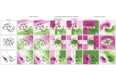
For a comaprison of the LogisticRegression with other classifiers see: Plot classification probability.
- decision_function(X)[source]#
Predict confidence scores for samples.
The confidence score for a sample is proportional to the signed distance of that sample to the hyperplane.
- Parameters:
- X{array-like, sparse matrix} of shape (n_samples, n_features)
The data matrix for which we want to get the confidence scores.
- Returns:
- scoresndarray of shape (n_samples,) or (n_samples, n_classes)
Confidence scores per
(n_samples, n_classes)combination. In the binary case, confidence score forself.classes_[1]where >0 means this class would be predicted.
- densify()[source]#
Convert coefficient matrix to dense array format.
Converts the
coef_member (back) to a numpy.ndarray. This is the default format ofcoef_and is required for fitting, so calling this method is only required on models that have previously been sparsified; otherwise, it is a no-op.- Returns:
- self
Fitted estimator.
- fit(X, y, sample_weight=None)[source]#
Fit the model according to the given training data.
- Parameters:
- X{array-like, sparse matrix} of shape (n_samples, n_features)
Training vector, where
n_samplesis the number of samples andn_featuresis the number of features.- yarray-like of shape (n_samples,)
Target vector relative to X.
- sample_weightarray-like of shape (n_samples,) default=None
Array of weights that are assigned to individual samples. If not provided, then each sample is given unit weight.
Added in version 0.17: sample_weight support to LogisticRegression.
- Returns:
- self
Fitted estimator.
Notes
The SAGA solver supports both float64 and float32 bit arrays.
- get_metadata_routing()[source]#
Get metadata routing of this object.
Please check User Guide on how the routing mechanism works.
- Returns:
- routingMetadataRequest
A
MetadataRequestencapsulating routing information.
- get_params(deep=True)[source]#
Get parameters for this estimator.
- Parameters:
- deepbool, default=True
If True, will return the parameters for this estimator and contained subobjects that are estimators.
- Returns:
- paramsdict
Parameter names mapped to their values.
- predict(X)[source]#
Predict class labels for samples in X.
- Parameters:
- X{array-like, sparse matrix} of shape (n_samples, n_features)
The data matrix for which we want to get the predictions.
- Returns:
- y_predndarray of shape (n_samples,)
Vector containing the class labels for each sample.
- predict_log_proba(X)[source]#
Predict logarithm of probability estimates.
The returned estimates for all classes are ordered by the label of classes.
- Parameters:
- Xarray-like of shape (n_samples, n_features)
Vector to be scored, where
n_samplesis the number of samples andn_featuresis the number of features.
- Returns:
- Tarray-like of shape (n_samples, n_classes)
Returns the log-probability of the sample for each class in the model, where classes are ordered as they are in
self.classes_.
- predict_proba(X)[source]#
Probability estimates.
The returned estimates for all classes are ordered by the label of classes.
For a multi_class problem, if multi_class is set to be “multinomial” the softmax function is used to find the predicted probability of each class. Else use a one-vs-rest approach, i.e. calculate the probability of each class assuming it to be positive using the logistic function and normalize these values across all the classes.
- Parameters:
- Xarray-like of shape (n_samples, n_features)
Vector to be scored, where
n_samplesis the number of samples andn_featuresis the number of features.
- Returns:
- Tarray-like of shape (n_samples, n_classes)
Returns the probability of the sample for each class in the model, where classes are ordered as they are in
self.classes_.
- score(X, y, sample_weight=None)[source]#
Return the mean accuracy on the given test data and labels.
In multi-label classification, this is the subset accuracy which is a harsh metric since you require for each sample that each label set be correctly predicted.
- Parameters:
- Xarray-like of shape (n_samples, n_features)
Test samples.
- yarray-like of shape (n_samples,) or (n_samples, n_outputs)
True labels for
X.- sample_weightarray-like of shape (n_samples,), default=None
Sample weights.
- Returns:
- scorefloat
Mean accuracy of
self.predict(X)w.r.t.y.
- set_fit_request(*, sample_weight: bool | None | str = '$UNCHANGED$') LogisticRegression[source]#
Request metadata passed to the
fitmethod.Note that this method is only relevant if
enable_metadata_routing=True(seesklearn.set_config). Please see User Guide on how the routing mechanism works.The options for each parameter are:
True: metadata is requested, and passed tofitif provided. The request is ignored if metadata is not provided.False: metadata is not requested and the meta-estimator will not pass it tofit.None: metadata is not requested, and the meta-estimator will raise an error if the user provides it.str: metadata should be passed to the meta-estimator with this given alias instead of the original name.
The default (
sklearn.utils.metadata_routing.UNCHANGED) retains the existing request. This allows you to change the request for some parameters and not others.Added in version 1.3.
Note
This method is only relevant if this estimator is used as a sub-estimator of a meta-estimator, e.g. used inside a
Pipeline. Otherwise it has no effect.- Parameters:
- sample_weightstr, True, False, or None, default=sklearn.utils.metadata_routing.UNCHANGED
Metadata routing for
sample_weightparameter infit.
- Returns:
- selfobject
The updated object.
- set_params(**params)[source]#
Set the parameters of this estimator.
The method works on simple estimators as well as on nested objects (such as
Pipeline). The latter have parameters of the form<component>__<parameter>so that it’s possible to update each component of a nested object.- Parameters:
- **paramsdict
Estimator parameters.
- Returns:
- selfestimator instance
Estimator instance.
- set_score_request(*, sample_weight: bool | None | str = '$UNCHANGED$') LogisticRegression[source]#
Request metadata passed to the
scoremethod.Note that this method is only relevant if
enable_metadata_routing=True(seesklearn.set_config). Please see User Guide on how the routing mechanism works.The options for each parameter are:
True: metadata is requested, and passed toscoreif provided. The request is ignored if metadata is not provided.False: metadata is not requested and the meta-estimator will not pass it toscore.None: metadata is not requested, and the meta-estimator will raise an error if the user provides it.str: metadata should be passed to the meta-estimator with this given alias instead of the original name.
The default (
sklearn.utils.metadata_routing.UNCHANGED) retains the existing request. This allows you to change the request for some parameters and not others.Added in version 1.3.
Note
This method is only relevant if this estimator is used as a sub-estimator of a meta-estimator, e.g. used inside a
Pipeline. Otherwise it has no effect.- Parameters:
- sample_weightstr, True, False, or None, default=sklearn.utils.metadata_routing.UNCHANGED
Metadata routing for
sample_weightparameter inscore.
- Returns:
- selfobject
The updated object.
- sparsify()[source]#
Convert coefficient matrix to sparse format.
Converts the
coef_member to a scipy.sparse matrix, which for L1-regularized models can be much more memory- and storage-efficient than the usual numpy.ndarray representation.The
intercept_member is not converted.- Returns:
- self
Fitted estimator.
Notes
For non-sparse models, i.e. when there are not many zeros in
coef_, this may actually increase memory usage, so use this method with care. A rule of thumb is that the number of zero elements, which can be computed with(coef_ == 0).sum(), must be more than 50% for this to provide significant benefits.After calling this method, further fitting with the partial_fit method (if any) will not work until you call densify.
Gallery examples#

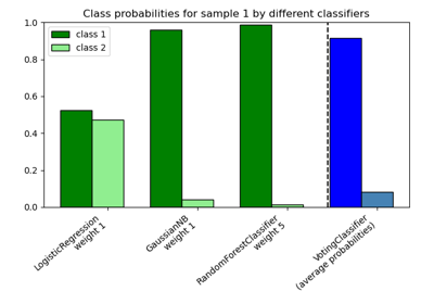
Plot class probabilities calculated by the VotingClassifier
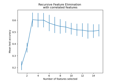
Recursive feature elimination with cross-validation

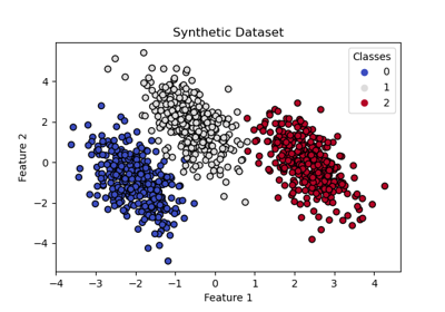
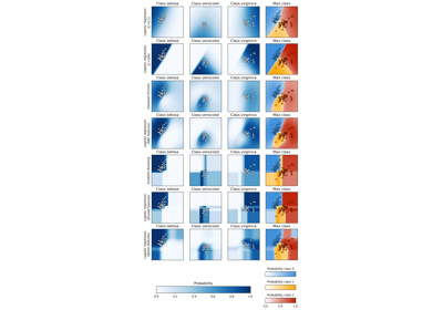
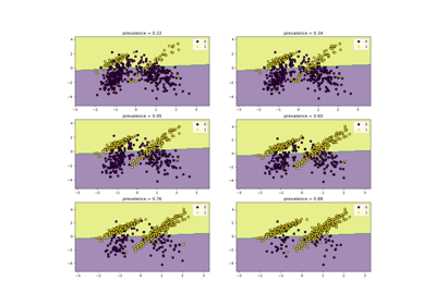
Decision Boundaries of Multinomial and One-vs-Rest Logistic Regression
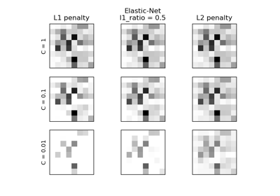
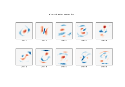
MNIST classification using multinomial logistic + L1
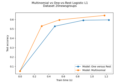
Multiclass sparse logistic regression on 20newgroups


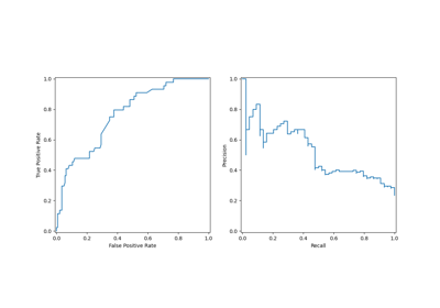
Class Likelihood Ratios to measure classification performance
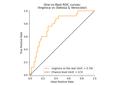
Multiclass Receiver Operating Characteristic (ROC)
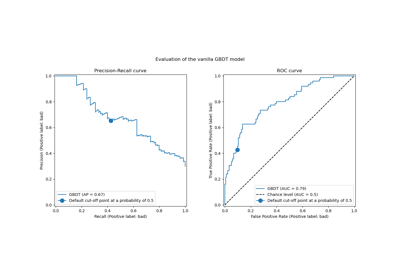
Post-hoc tuning the cut-off point of decision function
Post-tuning the decision threshold for cost-sensitive learning
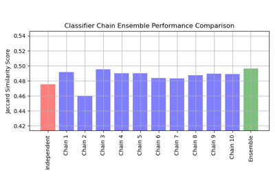
Multilabel classification using a classifier chain
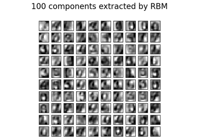
Restricted Boltzmann Machine features for digit classification
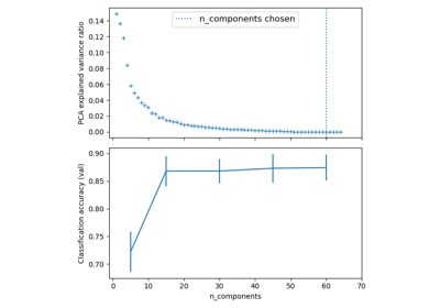
Pipelining: chaining a PCA and a logistic regression
Classification of text documents using sparse features