Ridge#
- class sklearn.linear_model.Ridge(alpha=1.0, *, fit_intercept=True, copy_X=True, max_iter=None, tol=0.0001, solver='auto', positive=False, random_state=None)[source]#
Linear least squares with l2 regularization.
Minimizes the objective function:
||y - Xw||^2_2 + alpha * ||w||^2_2
This model solves a regression model where the loss function is the linear least squares function and regularization is given by the l2-norm. Also known as Ridge Regression or Tikhonov regularization. This estimator has built-in support for multi-variate regression (i.e., when y is a 2d-array of shape (n_samples, n_targets)).
Read more in the User Guide.
- Parameters:
- alpha{float, ndarray of shape (n_targets,)}, default=1.0
Constant that multiplies the L2 term, controlling regularization strength.
alphamust be a non-negative float i.e. in[0, inf).When
alpha = 0, the objective is equivalent to ordinary least squares, solved by theLinearRegressionobject. For numerical reasons, usingalpha = 0with theRidgeobject is not advised. Instead, you should use theLinearRegressionobject.If an array is passed, penalties are assumed to be specific to the targets. Hence they must correspond in number.
- fit_interceptbool, default=True
Whether to fit the intercept for this model. If set to false, no intercept will be used in calculations (i.e.
Xandyare expected to be centered).- copy_Xbool, default=True
If True, X will be copied; else, it may be overwritten.
- max_iterint, default=None
Maximum number of iterations for conjugate gradient solver. For ‘sparse_cg’ and ‘lsqr’ solvers, the default value is determined by scipy.sparse.linalg. For ‘sag’ solver, the default value is 1000. For ‘lbfgs’ solver, the default value is 15000.
- tolfloat, default=1e-4
The precision of the solution (
coef_) is determined bytolwhich specifies a different convergence criterion for each solver:‘svd’:
tolhas no impact.‘cholesky’:
tolhas no impact.‘sparse_cg’: norm of residuals smaller than
tol.‘lsqr’:
tolis set as atol and btol of scipy.sparse.linalg.lsqr, which control the norm of the residual vector in terms of the norms of matrix and coefficients.‘sag’ and ‘saga’: relative change of coef smaller than
tol.‘lbfgs’: maximum of the absolute (projected) gradient=max|residuals| smaller than
tol.
Changed in version 1.2: Default value changed from 1e-3 to 1e-4 for consistency with other linear models.
- solver{‘auto’, ‘svd’, ‘cholesky’, ‘lsqr’, ‘sparse_cg’, ‘sag’, ‘saga’, ‘lbfgs’}, default=’auto’
Solver to use in the computational routines:
‘auto’ chooses the solver automatically based on the type of data.
‘svd’ uses a Singular Value Decomposition of X to compute the Ridge coefficients. It is the most stable solver, in particular more stable for singular matrices than ‘cholesky’ at the cost of being slower.
‘cholesky’ uses the standard
scipy.linalg.solvefunction to obtain a closed-form solution.‘sparse_cg’ uses the conjugate gradient solver as found in
scipy.sparse.linalg.cg. As an iterative algorithm, this solver is more appropriate than ‘cholesky’ for large-scale data (possibility to settolandmax_iter).‘lsqr’ uses the dedicated regularized least-squares routine
scipy.sparse.linalg.lsqr. It is the fastest and uses an iterative procedure.‘sag’ uses a Stochastic Average Gradient descent, and ‘saga’ uses its improved, unbiased version named SAGA. Both methods also use an iterative procedure, and are often faster than other solvers when both n_samples and n_features are large. Note that ‘sag’ and ‘saga’ fast convergence is only guaranteed on features with approximately the same scale. You can preprocess the data with a scaler from
sklearn.preprocessing.‘lbfgs’ uses L-BFGS-B algorithm implemented in
scipy.optimize.minimize. It can be used only whenpositiveis True.
All solvers except ‘svd’ support both dense and sparse data. However, only ‘lsqr’, ‘sag’, ‘sparse_cg’, and ‘lbfgs’ support sparse input when
fit_interceptis True.Added in version 0.17: Stochastic Average Gradient descent solver.
Added in version 0.19: SAGA solver.
- positivebool, default=False
When set to
True, forces the coefficients to be positive. Only ‘lbfgs’ solver is supported in this case.- random_stateint, RandomState instance, default=None
Used when
solver== ‘sag’ or ‘saga’ to shuffle the data. See Glossary for details.Added in version 0.17:
random_stateto support Stochastic Average Gradient.
- Attributes:
- coef_ndarray of shape (n_features,) or (n_targets, n_features)
Weight vector(s).
- intercept_float or ndarray of shape (n_targets,)
Independent term in decision function. Set to 0.0 if
fit_intercept = False.- n_iter_None or ndarray of shape (n_targets,)
Actual number of iterations for each target. Available only for ‘sag’ and ‘lsqr’ solvers. Other solvers will return None.
Added in version 0.17.
- n_features_in_int
Number of features seen during fit.
Added in version 0.24.
- feature_names_in_ndarray of shape (
n_features_in_,) Names of features seen during fit. Defined only when
Xhas feature names that are all strings.Added in version 1.0.
- solver_str
The solver that was used at fit time by the computational routines.
Added in version 1.5.
See also
RidgeClassifierRidge classifier.
RidgeCVRidge regression with built-in cross validation.
KernelRidgeKernel ridge regression combines ridge regression with the kernel trick.
Notes
Regularization improves the conditioning of the problem and reduces the variance of the estimates. Larger values specify stronger regularization. Alpha corresponds to
1 / (2C)in other linear models such asLogisticRegressionorLinearSVC.Examples
>>> from sklearn.linear_model import Ridge
>>> import numpy as np
>>> n_samples, n_features = 10, 5
>>> rng = np.random.RandomState(0)
>>> y = rng.randn(n_samples)
>>> X = rng.randn(n_samples, n_features)
>>> clf = Ridge(alpha=1.0)
>>> clf.fit(X, y)
Ridge()
- fit(X, y, sample_weight=None)[source]#
Fit Ridge regression model.
- Parameters:
- X{ndarray, sparse matrix} of shape (n_samples, n_features)
Training data.
- yndarray of shape (n_samples,) or (n_samples, n_targets)
Target values.
- sample_weightfloat or ndarray of shape (n_samples,), default=None
Individual weights for each sample. If given a float, every sample will have the same weight.
- Returns:
- selfobject
Fitted estimator.
- get_metadata_routing()[source]#
Get metadata routing of this object.
Please check User Guide on how the routing mechanism works.
- Returns:
- routingMetadataRequest
A
MetadataRequestencapsulating routing information.
- get_params(deep=True)[source]#
Get parameters for this estimator.
- Parameters:
- deepbool, default=True
If True, will return the parameters for this estimator and contained subobjects that are estimators.
- Returns:
- paramsdict
Parameter names mapped to their values.
- predict(X)[source]#
Predict using the linear model.
- Parameters:
- Xarray-like or sparse matrix, shape (n_samples, n_features)
Samples.
- Returns:
- Carray, shape (n_samples,)
Returns predicted values.
- score(X, y, sample_weight=None)[source]#
Return coefficient of determination on test data.
The coefficient of determination, \(R^2\), is defined as \((1 - \frac{u}{v})\), where \(u\) is the residual sum of squares
((y_true - y_pred)** 2).sum()and \(v\) is the total sum of squares((y_true - y_true.mean()) ** 2).sum(). The best possible score is 1.0 and it can be negative (because the model can be arbitrarily worse). A constant model that always predicts the expected value ofy, disregarding the input features, would get a \(R^2\) score of 0.0.- Parameters:
- Xarray-like of shape (n_samples, n_features)
Test samples. For some estimators this may be a precomputed kernel matrix or a list of generic objects instead with shape
(n_samples, n_samples_fitted), wheren_samples_fittedis the number of samples used in the fitting for the estimator.- yarray-like of shape (n_samples,) or (n_samples, n_outputs)
True values for
X.- sample_weightarray-like of shape (n_samples,), default=None
Sample weights.
- Returns:
- scorefloat
\(R^2\) of
self.predict(X)w.r.t.y.
Notes
The \(R^2\) score used when calling
scoreon a regressor usesmultioutput='uniform_average'from version 0.23 to keep consistent with default value ofr2_score. This influences thescoremethod of all the multioutput regressors (except forMultiOutputRegressor).
- set_fit_request(*, sample_weight: bool | None | str = '$UNCHANGED$') Ridge[source]#
Configure whether metadata should be requested to be passed to the
fitmethod.Note that this method is only relevant when this estimator is used as a sub-estimator within a meta-estimator and metadata routing is enabled with
enable_metadata_routing=True(seesklearn.set_config). Please check the User Guide on how the routing mechanism works.The options for each parameter are:
True: metadata is requested, and passed tofitif provided. The request is ignored if metadata is not provided.False: metadata is not requested and the meta-estimator will not pass it tofit.None: metadata is not requested, and the meta-estimator will raise an error if the user provides it.str: metadata should be passed to the meta-estimator with this given alias instead of the original name.
The default (
sklearn.utils.metadata_routing.UNCHANGED) retains the existing request. This allows you to change the request for some parameters and not others.Added in version 1.3.
- Parameters:
- sample_weightstr, True, False, or None, default=sklearn.utils.metadata_routing.UNCHANGED
Metadata routing for
sample_weightparameter infit.
- Returns:
- selfobject
The updated object.
- set_params(**params)[source]#
Set the parameters of this estimator.
The method works on simple estimators as well as on nested objects (such as
Pipeline). The latter have parameters of the form<component>__<parameter>so that it’s possible to update each component of a nested object.- Parameters:
- **paramsdict
Estimator parameters.
- Returns:
- selfestimator instance
Estimator instance.
- set_score_request(*, sample_weight: bool | None | str = '$UNCHANGED$') Ridge[source]#
Configure whether metadata should be requested to be passed to the
scoremethod.Note that this method is only relevant when this estimator is used as a sub-estimator within a meta-estimator and metadata routing is enabled with
enable_metadata_routing=True(seesklearn.set_config). Please check the User Guide on how the routing mechanism works.The options for each parameter are:
True: metadata is requested, and passed toscoreif provided. The request is ignored if metadata is not provided.False: metadata is not requested and the meta-estimator will not pass it toscore.None: metadata is not requested, and the meta-estimator will raise an error if the user provides it.str: metadata should be passed to the meta-estimator with this given alias instead of the original name.
The default (
sklearn.utils.metadata_routing.UNCHANGED) retains the existing request. This allows you to change the request for some parameters and not others.Added in version 1.3.
- Parameters:
- sample_weightstr, True, False, or None, default=sklearn.utils.metadata_routing.UNCHANGED
Metadata routing for
sample_weightparameter inscore.
- Returns:
- selfobject
The updated object.
Gallery examples#
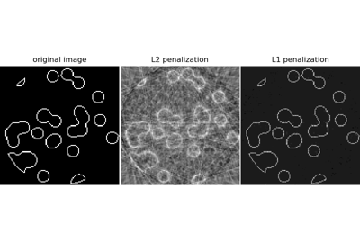
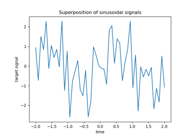
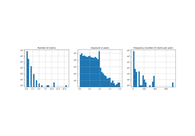
Compressive sensing: tomography reconstruction with L1 prior (Lasso)
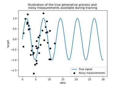
Comparison of kernel ridge and Gaussian process regression
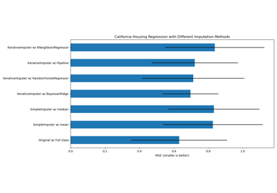
Imputing missing values with variants of IterativeImputer
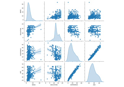
Common pitfalls in the interpretation of coefficients of linear models
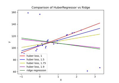
HuberRegressor vs Ridge on dataset with strong outliers

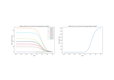
Ridge coefficients as a function of the L2 Regularization
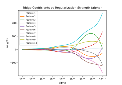
Plot Ridge coefficients as a function of the regularization