Note
Go to the end to download the full example code or to run this example in your browser via JupyterLite or Binder.
Comparison of kernel ridge and Gaussian process regression#
This example illustrates differences between a kernel ridge regression and a Gaussian process regression.
Both kernel ridge regression and Gaussian process regression are using a so-called “kernel trick” to make their models expressive enough to fit the training data. However, the machine learning problems solved by the two methods are drastically different.
Kernel ridge regression will find the target function that minimizes a loss function (the mean squared error).
Instead of finding a single target function, the Gaussian process regression employs a probabilistic approach : a Gaussian posterior distribution over target functions is defined based on the Bayes’ theorem, Thus prior probabilities on target functions are being combined with a likelihood function defined by the observed training data to provide estimates of the posterior distributions.
We will illustrate these differences with an example and we will also focus on tuning the kernel hyperparameters.
# Authors: The scikit-learn developers
# SPDX-License-Identifier: BSD-3-Clause
Generating a dataset#
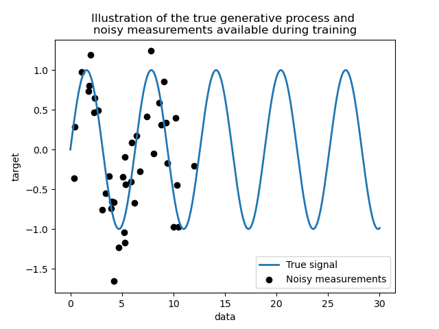
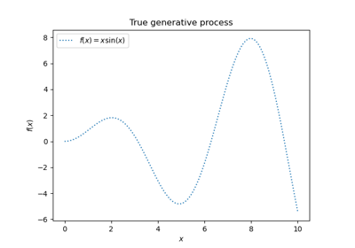
We create a synthetic dataset. The true generative process will take a 1-D vector and compute its sine. Note that the period of this sine is thus \(2 \pi\). We will reuse this information later in this example.
import numpy as np

rng = np.random.RandomState(0)
data = np.linspace(0, 30, num=1_000).reshape(-1, 1)
target = np.sin(data).ravel()
Now, we can imagine a scenario where we get observations from this true process. However, we will add some challenges:
the measurements will be noisy;
only samples from the beginning of the signal will be available.
training_sample_indices = rng.choice(np.arange(0, 400), size=40, replace=False)
training_data = data[training_sample_indices]
training_noisy_target = target[training_sample_indices] + 0.5 * rng.randn(
    len(training_sample_indices)
)
Let’s plot the true signal and the noisy measurements available for training.
import matplotlib.pyplot as plt

plt.plot(data, target, label="True signal", linewidth=2)
plt.scatter(
    training_data,
    training_noisy_target,
    color="black",
    label="Noisy measurements",
)
plt.legend()
plt.xlabel("data")
plt.ylabel("target")
_ = plt.title(
    "Illustration of the true generative process and \n"
    "noisy measurements available during training"
)
Limitations of a simple linear model#
First, we would like to highlight the limitations of a linear model given
our dataset. We fit a Ridge and check the
predictions of this model on our dataset.
from sklearn.linear_model import Ridge

ridge = Ridge().fit(training_data, training_noisy_target)

plt.plot(data, target, label="True signal", linewidth=2)
plt.scatter(
    training_data,
    training_noisy_target,
    color="black",
    label="Noisy measurements",
)
plt.plot(data, ridge.predict(data), label="Ridge regression")
plt.legend()
plt.xlabel("data")
plt.ylabel("target")
_ = plt.title("Limitation of a linear model such as ridge")
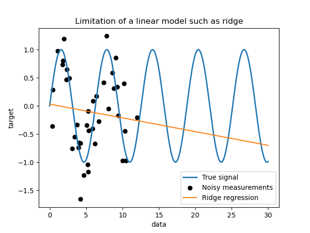
Such a ridge regressor underfits data since it is not expressive enough.
Kernel methods: kernel ridge and Gaussian process#
Kernel ridge#
We can make the previous linear model more expressive by using a so-called kernel. A kernel is an embedding from the original feature space to another one. Simply put, it is used to map our original data into a newer and more complex feature space. This new space is explicitly defined by the choice of kernel.
In our case, we know that the true generative process is a periodic function.
We can use a ExpSineSquared kernel
which allows recovering the periodicity. The class
KernelRidge will accept such a kernel.
Using this model together with a kernel is equivalent to embed the data using the mapping function of the kernel and then apply a ridge regression. In practice, the data are not mapped explicitly; instead the dot product between samples in the higher dimensional feature space is computed using the “kernel trick”.
Thus, let’s use such a KernelRidge.
import time

from sklearn.gaussian_process.kernels import ExpSineSquared
from sklearn.kernel_ridge import KernelRidge

kernel_ridge = KernelRidge(kernel=ExpSineSquared())

start_time = time.time()
kernel_ridge.fit(training_data, training_noisy_target)
print(
    f"Fitting KernelRidge with default kernel: {time.time() - start_time:.3f} seconds"
)
Fitting KernelRidge with default kernel: 0.001 seconds
plt.plot(data, target, label="True signal", linewidth=2, linestyle="dashed")
plt.scatter(
    training_data,
    training_noisy_target,
    color="black",
    label="Noisy measurements",
)
plt.plot(
    data,
    kernel_ridge.predict(data),
    label="Kernel ridge",
    linewidth=2,
    linestyle="dashdot",
)
plt.legend(loc="lower right")
plt.xlabel("data")
plt.ylabel("target")
_ = plt.title(
    "Kernel ridge regression with an exponential sine squared\n "
    "kernel using default hyperparameters"
)
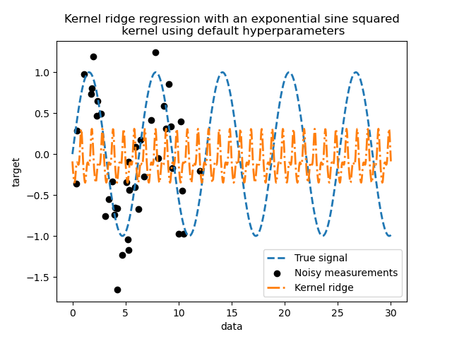
This fitted model is not accurate. Indeed, we did not set the parameters of the kernel and instead used the default ones. We can inspect them.
kernel_ridge.kernel
ExpSineSquared(length_scale=1, periodicity=1)
Our kernel has two parameters: the length-scale and the periodicity. For our
dataset, we use sin as the generative process, implying a
\(2 \pi\)-periodicity for the signal. The default value of the parameter
being \(1\), it explains the high frequency observed in the predictions of
our model.
Similar conclusions could be drawn with the length-scale parameter. Thus, it
tells us that the kernel parameters need to be tuned. We will use a randomized
search to tune the different parameters the kernel ridge model: the alpha
parameter and the kernel parameters.
from scipy.stats import loguniform

from sklearn.model_selection import RandomizedSearchCV

param_distributions = {
    "alpha": loguniform(1e0, 1e3),
    "kernel__length_scale": loguniform(1e-2, 1e2),
    "kernel__periodicity": loguniform(1e0, 1e1),
}
kernel_ridge_tuned = RandomizedSearchCV(
    kernel_ridge,
    param_distributions=param_distributions,
    n_iter=500,
    random_state=0,
)
start_time = time.time()
kernel_ridge_tuned.fit(training_data, training_noisy_target)
print(f"Time for KernelRidge fitting: {time.time() - start_time:.3f} seconds")
Time for KernelRidge fitting: 4.956 seconds
Fitting the model is now more computationally expensive since we have to try several combinations of hyperparameters. We can have a look at the hyperparameters found to get some intuitions.
kernel_ridge_tuned.best_params_
{'alpha': np.float64(1.991584977345022), 'kernel__length_scale': np.float64(0.7986499491396734), 'kernel__periodicity': np.float64(6.6072758064261095)}
Looking at the best parameters, we see that they are different from the defaults. We also see that the periodicity is closer to the expected value: \(2 \pi\). We can now inspect the predictions of our tuned kernel ridge.
Time for KernelRidge predict: 0.002 seconds
plt.plot(data, target, label="True signal", linewidth=2, linestyle="dashed")
plt.scatter(
    training_data,
    training_noisy_target,
    color="black",
    label="Noisy measurements",
)
plt.plot(
    data,
    predictions_kr,
    label="Kernel ridge",
    linewidth=2,
    linestyle="dashdot",
)
plt.legend(loc="lower right")
plt.xlabel("data")
plt.ylabel("target")
_ = plt.title(
    "Kernel ridge regression with an exponential sine squared\n "
    "kernel using tuned hyperparameters"
)
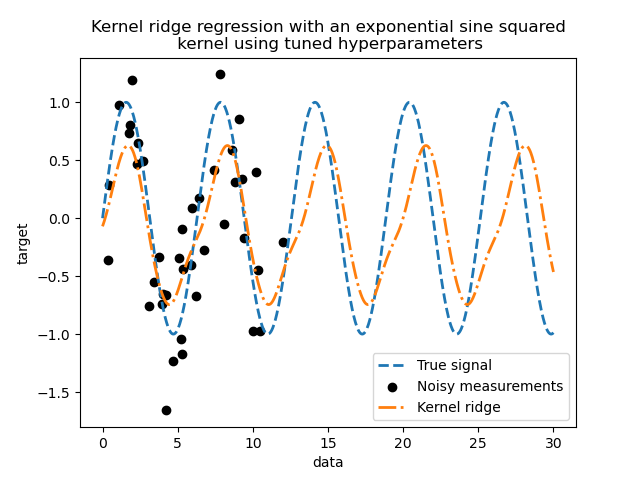
We get a much more accurate model. We still observe some errors mainly due to the noise added to the dataset.
Gaussian process regression#
Now, we will use a
GaussianProcessRegressor to fit the same
dataset. When training a Gaussian process, the hyperparameters of the kernel
are optimized during the fitting process. There is no need for an external
hyperparameter search. Here, we create a slightly more complex kernel than
for the kernel ridge regressor: we add a
WhiteKernel that is used to
estimate the noise in the dataset.
from sklearn.gaussian_process import GaussianProcessRegressor
from sklearn.gaussian_process.kernels import WhiteKernel

kernel = 1.0 * ExpSineSquared(1.0, 5.0, periodicity_bounds=(1e-2, 1e1)) + WhiteKernel(
    1e-1
)
gaussian_process = GaussianProcessRegressor(kernel=kernel)
start_time = time.time()
gaussian_process.fit(training_data, training_noisy_target)
print(
    f"Time for GaussianProcessRegressor fitting: {time.time() - start_time:.3f} seconds"
)
Time for GaussianProcessRegressor fitting: 0.039 seconds
The computation cost of training a Gaussian process is much less than the kernel ridge that uses a randomized search. We can check the parameters of the kernels that we computed.
gaussian_process.kernel_
0.675**2 * ExpSineSquared(length_scale=1.34, periodicity=6.57) + WhiteKernel(noise_level=0.182)
Indeed, we see that the parameters have been optimized. Looking at the
periodicity parameter, we see that we found a period close to the
theoretical value \(2 \pi\). We can have a look now at the predictions of
our model.
Time for GaussianProcessRegressor predict: 0.003 seconds
plt.plot(data, target, label="True signal", linewidth=2, linestyle="dashed")
plt.scatter(
    training_data,
    training_noisy_target,
    color="black",
    label="Noisy measurements",
)
# Plot the predictions of the kernel ridge
plt.plot(
    data,
    predictions_kr,
    label="Kernel ridge",
    linewidth=2,
    linestyle="dashdot",
)
# Plot the predictions of the gaussian process regressor
plt.plot(
    data,
    mean_predictions_gpr,
    label="Gaussian process regressor",
    linewidth=2,
    linestyle="dotted",
)
plt.fill_between(
    data.ravel(),
    mean_predictions_gpr - std_predictions_gpr,
    mean_predictions_gpr + std_predictions_gpr,
    color="tab:green",
    alpha=0.2,
)
plt.legend(loc="lower right")
plt.xlabel("data")
plt.ylabel("target")
_ = plt.title("Comparison between kernel ridge and gaussian process regressor")
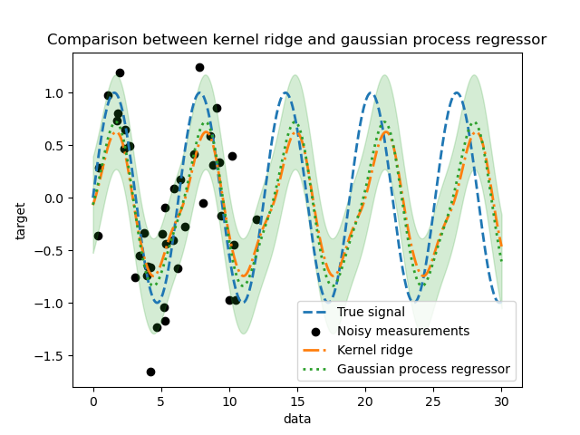
We observe that the results of the kernel ridge and the Gaussian process regressor are close. However, the Gaussian process regressor also provide an uncertainty information that is not available with a kernel ridge. Due to the probabilistic formulation of the target functions, the Gaussian process can output the standard deviation (or the covariance) together with the mean predictions of the target functions.
However, it comes at a cost: the time to compute the predictions is higher with a Gaussian process.
Final conclusion#
We can give a final word regarding the possibility of the two models to extrapolate. Indeed, we only provided the beginning of the signal as a training set. Using a periodic kernel forces our model to repeat the pattern found on the training set. Using this kernel information together with the capacity of the both models to extrapolate, we observe that the models will continue to predict the sine pattern.
Gaussian process allows to combine kernels together. Thus, we could associate the exponential sine squared kernel together with a radial basis function kernel.
from sklearn.gaussian_process.kernels import RBF

kernel = 1.0 * ExpSineSquared(1.0, 5.0, periodicity_bounds=(1e-2, 1e1)) * RBF(
    length_scale=15, length_scale_bounds="fixed"
) + WhiteKernel(1e-1)
gaussian_process = GaussianProcessRegressor(kernel=kernel)
gaussian_process.fit(training_data, training_noisy_target)
mean_predictions_gpr, std_predictions_gpr = gaussian_process.predict(
    data,
    return_std=True,
)
plt.plot(data, target, label="True signal", linewidth=2, linestyle="dashed")
plt.scatter(
    training_data,
    training_noisy_target,
    color="black",
    label="Noisy measurements",
)
# Plot the predictions of the kernel ridge
plt.plot(
    data,
    predictions_kr,
    label="Kernel ridge",
    linewidth=2,
    linestyle="dashdot",
)
# Plot the predictions of the gaussian process regressor
plt.plot(
    data,
    mean_predictions_gpr,
    label="Gaussian process regressor",
    linewidth=2,
    linestyle="dotted",
)
plt.fill_between(
    data.ravel(),
    mean_predictions_gpr - std_predictions_gpr,
    mean_predictions_gpr + std_predictions_gpr,
    color="tab:green",
    alpha=0.2,
)
plt.legend(loc="lower right")
plt.xlabel("data")
plt.ylabel("target")
_ = plt.title("Effect of using a radial basis function kernel")
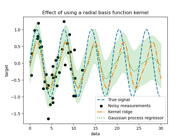
The effect of using a radial basis function kernel will attenuate the periodicity effect once that no sample are available in the training. As testing samples get further away from the training ones, predictions are converging towards their mean and their standard deviation also increases.
Total running time of the script: (0 minutes 5.750 seconds)
Related examples
Gaussian Processes regression: basic introductory example
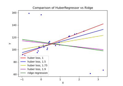
HuberRegressor vs Ridge on dataset with strong outliers

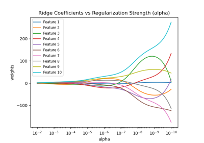
Plot Ridge coefficients as a function of the regularization
