Note
Go to the end to download the full example code or to run this example in your browser via JupyterLite or Binder.
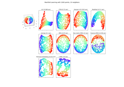
Comparison of Manifold Learning methods#
An illustration of dimensionality reduction on the S-curve dataset with various manifold learning methods.
For a discussion and comparison of these algorithms, see the manifold module page
For a similar example, where the methods are applied to a sphere dataset, see Manifold Learning methods on a severed sphere
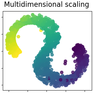
Note that the purpose of the MDS is to find a low-dimensional representation of the data (here 2D) in which the distances respect well the distances in the original high-dimensional space, unlike other manifold-learning algorithms, it does not seeks an isotropic representation of the data in the low-dimensional space.
# Authors: The scikit-learn developers
# SPDX-License-Identifier: BSD-3-Clause
Dataset preparation#
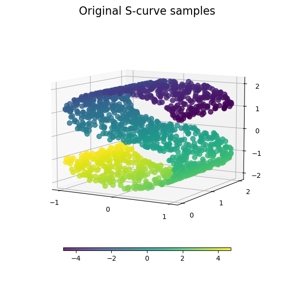
We start by generating the S-curve dataset.
import matplotlib.pyplot as plt

# unused but required import for doing 3d projections with matplotlib < 3.2
import mpl_toolkits.mplot3d  # noqa: F401
from matplotlib import ticker

from sklearn import datasets, manifold

n_samples = 1500
S_points, S_color = datasets.make_s_curve(n_samples, random_state=0)
Let’s look at the original data. Also define some helping functions, which we will use further on.
def plot_3d(points, points_color, title):
    x, y, z = points.T

    fig, ax = plt.subplots(
        figsize=(6, 6),
        facecolor="white",
        tight_layout=True,
        subplot_kw={"projection": "3d"},
    )
    fig.suptitle(title, size=16)
    col = ax.scatter(x, y, z, c=points_color, s=50, alpha=0.8)
    ax.view_init(azim=-60, elev=9)
    ax.xaxis.set_major_locator(ticker.MultipleLocator(1))
    ax.yaxis.set_major_locator(ticker.MultipleLocator(1))
    ax.zaxis.set_major_locator(ticker.MultipleLocator(1))

    fig.colorbar(col, ax=ax, orientation="horizontal", shrink=0.6, aspect=60, pad=0.01)
    plt.show()


def plot_2d(points, points_color, title):
    fig, ax = plt.subplots(figsize=(3, 3), facecolor="white", constrained_layout=True)
    fig.suptitle(title, size=16)
    add_2d_scatter(ax, points, points_color)
    plt.show()


def add_2d_scatter(ax, points, points_color, title=None):
    x, y = points.T
    ax.scatter(x, y, c=points_color, s=50, alpha=0.8)
    ax.set_title(title)
    ax.xaxis.set_major_formatter(ticker.NullFormatter())
    ax.yaxis.set_major_formatter(ticker.NullFormatter())


plot_3d(S_points, S_color, "Original S-curve samples")
Define algorithms for the manifold learning#
Manifold learning is an approach to non-linear dimensionality reduction. Algorithms for this task are based on the idea that the dimensionality of many data sets is only artificially high.
Read more in the User Guide.
n_neighbors = 12  # neighborhood which is used to recover the locally linear structure
n_components = 2  # number of coordinates for the manifold
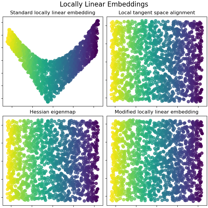
Locally Linear Embeddings#
Locally linear embedding (LLE) can be thought of as a series of local Principal Component Analyses which are globally compared to find the best non-linear embedding. Read more in the User Guide.
params = {
    "n_neighbors": n_neighbors,
    "n_components": n_components,
    "eigen_solver": "auto",
    "random_state": 0,
}

lle_standard = manifold.LocallyLinearEmbedding(method="standard", **params)
S_standard = lle_standard.fit_transform(S_points)

lle_ltsa = manifold.LocallyLinearEmbedding(method="ltsa", **params)
S_ltsa = lle_ltsa.fit_transform(S_points)

lle_hessian = manifold.LocallyLinearEmbedding(method="hessian", **params)
S_hessian = lle_hessian.fit_transform(S_points)

lle_mod = manifold.LocallyLinearEmbedding(method="modified", **params)
S_mod = lle_mod.fit_transform(S_points)
fig, axs = plt.subplots(
    nrows=2, ncols=2, figsize=(7, 7), facecolor="white", constrained_layout=True
)
fig.suptitle("Locally Linear Embeddings", size=16)

lle_methods = [
    ("Standard locally linear embedding", S_standard),
    ("Local tangent space alignment", S_ltsa),
    ("Hessian eigenmap", S_hessian),
    ("Modified locally linear embedding", S_mod),
]
for ax, method in zip(axs.flat, lle_methods):
    name, points = method
    add_2d_scatter(ax, points, S_color, name)

plt.show()
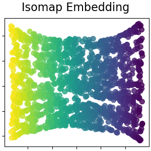
Isomap Embedding#
Non-linear dimensionality reduction through Isometric Mapping. Isomap seeks a lower-dimensional embedding which maintains geodesic distances between all points. Read more in the User Guide.
isomap = manifold.Isomap(n_neighbors=n_neighbors, n_components=n_components, p=1)
S_isomap = isomap.fit_transform(S_points)

plot_2d(S_isomap, S_color, "Isomap Embedding")
Multidimensional scaling#
Multidimensional scaling (MDS) seeks a low-dimensional representation of the data in which the distances respect well the distances in the original high-dimensional space. Read more in the User Guide.
md_scaling = manifold.MDS(
    n_components=n_components,
    max_iter=50,
    n_init=1,
    random_state=0,
    init="classical_mds",
    normalized_stress=False,
)
S_scaling_metric = md_scaling.fit_transform(S_points)

md_scaling_nonmetric = manifold.MDS(
    n_components=n_components,
    max_iter=50,
    n_init=1,
    random_state=0,
    normalized_stress=False,
    metric_mds=False,
    init="classical_mds",
)
S_scaling_nonmetric = md_scaling_nonmetric.fit_transform(S_points)

md_scaling_classical = manifold.ClassicalMDS(n_components=n_components)
S_scaling_classical = md_scaling_classical.fit_transform(S_points)
fig, axs = plt.subplots(
    nrows=1, ncols=3, figsize=(7, 3.5), facecolor="white", constrained_layout=True
)
fig.suptitle("Multidimensional scaling", size=16)

mds_methods = [
    ("Metric MDS", S_scaling_metric),
    ("Non-metric MDS", S_scaling_nonmetric),
    ("Classical MDS", S_scaling_classical),
]
for ax, method in zip(axs.flat, mds_methods):
    name, points = method
    add_2d_scatter(ax, points, S_color, name)

plt.show()
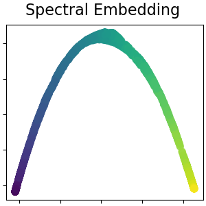
Spectral embedding for non-linear dimensionality reduction#
This implementation uses Laplacian Eigenmaps, which finds a low dimensional representation of the data using a spectral decomposition of the graph Laplacian. Read more in the User Guide.
spectral = manifold.SpectralEmbedding(
    n_components=n_components, n_neighbors=n_neighbors, random_state=42
)
S_spectral = spectral.fit_transform(S_points)

plot_2d(S_spectral, S_color, "Spectral Embedding")
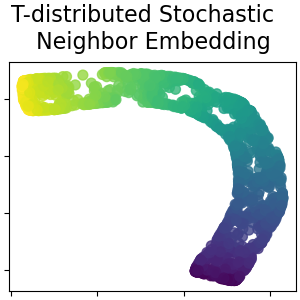
T-distributed Stochastic Neighbor Embedding#
It converts similarities between data points to joint probabilities and tries to minimize the Kullback-Leibler divergence between the joint probabilities of the low-dimensional embedding and the high-dimensional data. t-SNE has a cost function that is not convex, i.e. with different initializations we can get different results. Read more in the User Guide.
t_sne = manifold.TSNE(
    n_components=n_components,
    perplexity=30,
    init="random",
    max_iter=250,
    random_state=0,
)
S_t_sne = t_sne.fit_transform(S_points)

plot_2d(S_t_sne, S_color, "T-distributed Stochastic  \n Neighbor Embedding")
Total running time of the script: (0 minutes 18.855 seconds)
Related examples
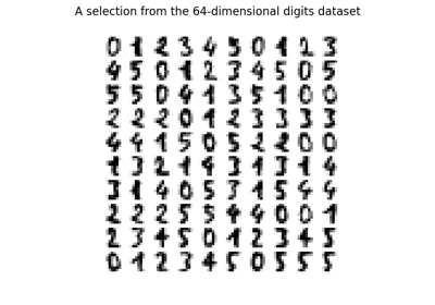
Manifold learning on handwritten digits: Locally Linear Embedding, Isomap…