Note
Go to the end to download the full example code or to run this example in your browser via JupyterLite or Binder.
Vector Quantization Example#
This example shows how one can use KBinsDiscretizer
to perform vector quantization on a set of toy image, the raccoon face.
# Authors: The scikit-learn developers
# SPDX-License-Identifier: BSD-3-Clause
Original image#
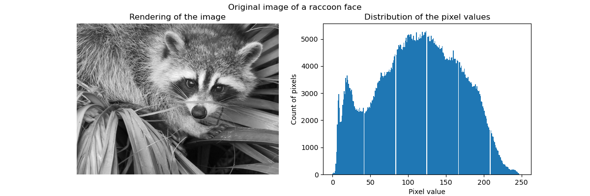
We start by loading the raccoon face image from SciPy. We will additionally check a couple of information regarding the image, such as the shape and data type used to store the image.
The dimension of the image is (768, 1024)
The data used to encode the image is of type uint8
The number of bytes taken in RAM is 786432
Thus the image is a 2D array of 768 pixels in height and 1024 pixels in width. Each value is a 8-bit unsigned integer, which means that the image is encoded using 8 bits per pixel. The total memory usage of the image is 786 kilobytes (1 byte equals 8 bits).
Using 8-bit unsigned integer means that the image is encoded using 256 different shades of gray, at most. We can check the distribution of these values.
import matplotlib.pyplot as plt

fig, ax = plt.subplots(ncols=2, figsize=(12, 4))

ax[0].imshow(raccoon_face, cmap=plt.cm.gray)
ax[0].axis("off")
ax[0].set_title("Rendering of the image")
ax[1].hist(raccoon_face.ravel(), bins=256)
ax[1].set_xlabel("Pixel value")
ax[1].set_ylabel("Count of pixels")
ax[1].set_title("Distribution of the pixel values")
_ = fig.suptitle("Original image of a raccoon face")
Compression via vector quantization#
The idea behind compression via vector quantization is to reduce the number of gray levels to represent an image. For instance, we can use 8 values instead of 256 values. Therefore, it means that we could efficiently use 3 bits instead of 8 bits to encode a single pixel and therefore reduce the memory usage by a factor of approximately 2.5. We will later discuss about this memory usage.
Encoding strategy#
The compression can be done using a
KBinsDiscretizer. We need to choose a strategy
to define the 8 gray values to sub-sample. The simplest strategy is to define
them equally spaced, which correspond to setting strategy="uniform". From
the previous histogram, we know that this strategy is certainly not optimal.
from sklearn.preprocessing import KBinsDiscretizer

n_bins = 8
encoder = KBinsDiscretizer(
    n_bins=n_bins,
    encode="ordinal",
    strategy="uniform",
    random_state=0,
)
compressed_raccoon_uniform = encoder.fit_transform(raccoon_face.reshape(-1, 1)).reshape(
    raccoon_face.shape
)

fig, ax = plt.subplots(ncols=2, figsize=(12, 4))
ax[0].imshow(compressed_raccoon_uniform, cmap=plt.cm.gray)
ax[0].axis("off")
ax[0].set_title("Rendering of the image")
ax[1].hist(compressed_raccoon_uniform.ravel(), bins=256)
ax[1].set_xlabel("Pixel value")
ax[1].set_ylabel("Count of pixels")
ax[1].set_title("Sub-sampled distribution of the pixel values")
_ = fig.suptitle("Raccoon face compressed using 3 bits and a uniform strategy")
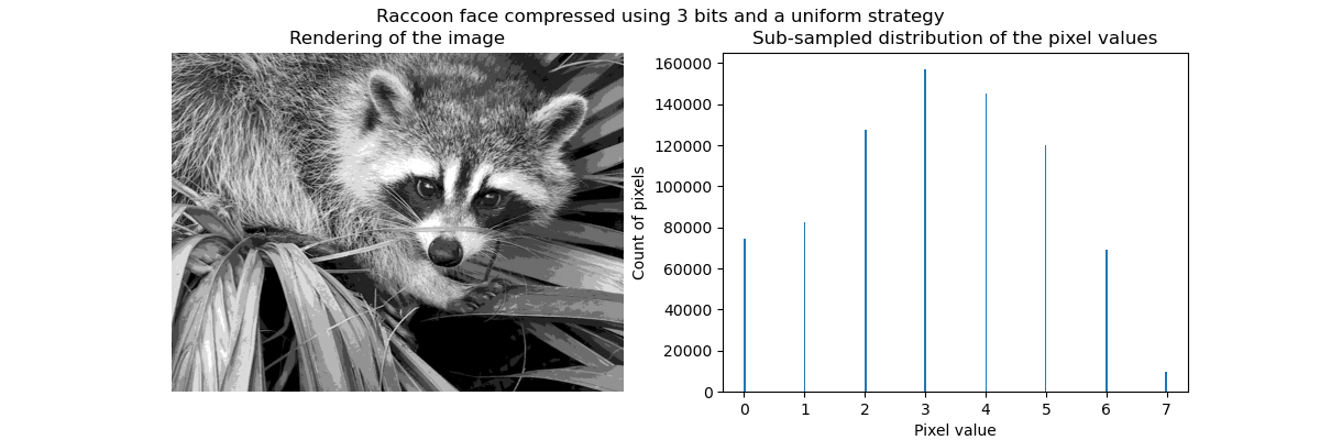
Qualitatively, we can spot some small regions where we see the effect of the compression (e.g. leaves on the bottom right corner). But after all, the resulting image is still looking good.
We observe that the distribution of pixels values have been mapped to 8 different values. We can check the correspondence between such values and the original pixel values.
bin_edges = encoder.bin_edges_[0]
bin_center = bin_edges[:-1] + (bin_edges[1:] - bin_edges[:-1]) / 2
bin_center
array([ 15.5625,  46.6875,  77.8125, 108.9375, 140.0625, 171.1875,
       202.3125, 233.4375])
_, ax = plt.subplots()
ax.hist(raccoon_face.ravel(), bins=256)
color = "tab:orange"
for center in bin_center:
    ax.axvline(center, color=color)
    ax.text(center - 10, ax.get_ybound()[1] + 100, f"{center:.1f}", color=color)
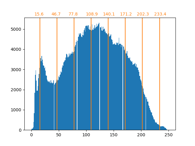
As previously stated, the uniform sampling strategy is not optimal. Notice for instance that the pixels mapped to the value 7 will encode a rather small amount of information, whereas the mapped value 3 will represent a large amount of counts. We can instead use a clustering strategy such as k-means to find a more optimal mapping.
encoder = KBinsDiscretizer(
n_bins=n_bins,
encode="ordinal",
strategy="kmeans",
random_state=0,
)
compressed_raccoon_kmeans = encoder.fit_transform(raccoon_face.reshape(-1, 1)).reshape(
raccoon_face.shape
)
fig, ax = plt.subplots(ncols=2, figsize=(12, 4))
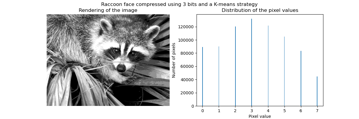
ax[0].imshow(compressed_raccoon_kmeans, cmap=plt.cm.gray)
ax[0].axis("off")
ax[0].set_title("Rendering of the image")
ax[1].hist(compressed_raccoon_kmeans.ravel(), bins=256)
ax[1].set_xlabel("Pixel value")
ax[1].set_ylabel("Number of pixels")
ax[1].set_title("Distribution of the pixel values")
_ = fig.suptitle("Raccoon face compressed using 3 bits and a K-means strategy")
bin_edges = encoder.bin_edges_[0]
bin_center = bin_edges[:-1] + (bin_edges[1:] - bin_edges[:-1]) / 2
bin_center
array([ 18.90934343,  53.33478066,  82.59678424, 109.22385188,
       134.67876527, 159.67877978, 184.72384803, 223.17132867])
_, ax = plt.subplots()
ax.hist(raccoon_face.ravel(), bins=256)
color = "tab:orange"
for center in bin_center:
    ax.axvline(center, color=color)
    ax.text(center - 10, ax.get_ybound()[1] + 100, f"{center:.1f}", color=color)

The counts in the bins are now more balanced and their centers are no longer
equally spaced. Note that we could enforce the same number of pixels per bin
by using the strategy="quantile" instead of strategy="kmeans".
Memory footprint#
We previously stated that we should save 8 times less memory. Let’s verify it.
print(f"The number of bytes taken in RAM is {compressed_raccoon_kmeans.nbytes}")
print(f"Compression ratio: {compressed_raccoon_kmeans.nbytes / raccoon_face.nbytes}")
The number of bytes taken in RAM is 6291456
Compression ratio: 8.0
It is quite surprising to see that our compressed image is taking x8 more memory than the original image. This is indeed the opposite of what we expected. The reason is mainly due to the type of data used to encode the image.
print(f"Type of the compressed image: {compressed_raccoon_kmeans.dtype}")
Type of the compressed image: float64
Indeed, the output of the KBinsDiscretizer is
an array of 64-bit float. It means that it takes x8 more memory. However, we
use this 64-bit float representation to encode 8 values. Indeed, we will save
memory only if we cast the compressed image into an array of 3-bits integers. We
could use the method numpy.ndarray.astype. However, a 3-bits integer
representation does not exist and to encode the 8 values, we would need to use
the 8-bit unsigned integer representation as well.
In practice, observing a memory gain would require the original image to be in a 64-bit float representation.
Total running time of the script: (0 minutes 2.096 seconds)
Related examples
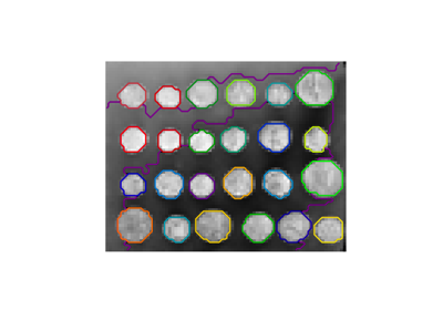
A demo of structured Ward hierarchical clustering on an image of coins