Note
Go to the end to download the full example code or to run this example in your browser via JupyterLite or Binder.
Demonstration of k-means assumptions#
This example is meant to illustrate situations where k-means produces unintuitive and possibly undesirable clusters.
# Authors: The scikit-learn developers
# SPDX-License-Identifier: BSD-3-Clause
Data generation#
The function make_blobs generates isotropic
(spherical) gaussian blobs. To obtain anisotropic (elliptical) gaussian blobs
one has to define a linear transformation.
import numpy as np

from sklearn.datasets import make_blobs

n_samples = 1500
random_state = 170
transformation = [[0.60834549, -0.63667341], [-0.40887718, 0.85253229]]

X, y = make_blobs(n_samples=n_samples, random_state=random_state)
X_aniso = np.dot(X, transformation)  # Anisotropic blobs
X_varied, y_varied = make_blobs(
    n_samples=n_samples, cluster_std=[1.0, 2.5, 0.5], random_state=random_state
)  # Unequal variance
X_filtered = np.vstack(
    (X[y == 0][:500], X[y == 1][:100], X[y == 2][:10])
)  # Unevenly sized blobs
y_filtered = [0] * 500 + [1] * 100 + [2] * 10
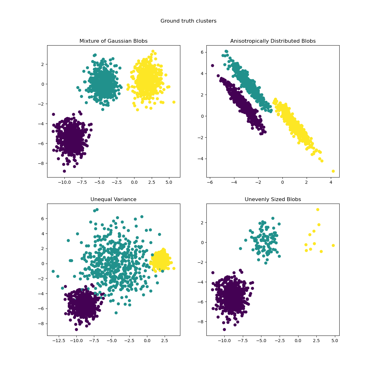
We can visualize the resulting data:
import matplotlib.pyplot as plt

fig, axs = plt.subplots(nrows=2, ncols=2, figsize=(12, 12))

axs[0, 0].scatter(X[:, 0], X[:, 1], c=y)
axs[0, 0].set_title("Mixture of Gaussian Blobs")

axs[0, 1].scatter(X_aniso[:, 0], X_aniso[:, 1], c=y)
axs[0, 1].set_title("Anisotropically Distributed Blobs")

axs[1, 0].scatter(X_varied[:, 0], X_varied[:, 1], c=y_varied)
axs[1, 0].set_title("Unequal Variance")

axs[1, 1].scatter(X_filtered[:, 0], X_filtered[:, 1], c=y_filtered)
axs[1, 1].set_title("Unevenly Sized Blobs")

plt.suptitle("Ground truth clusters").set_y(0.95)
plt.show()
Fit models and plot results#
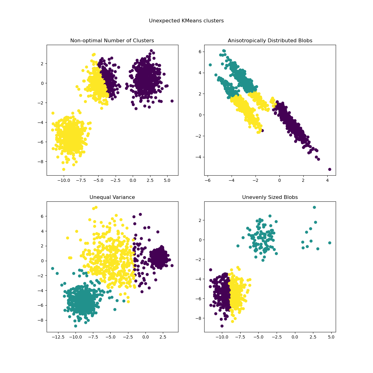
The previously generated data is now used to show how
KMeans behaves in the following scenarios:
Non-optimal number of clusters: in a real setting there is no uniquely defined true number of clusters. An appropriate number of clusters has to be decided from data-based criteria and knowledge of the intended goal.
Anisotropically distributed blobs: k-means consists of minimizing sample’s euclidean distances to the centroid of the cluster they are assigned to. As a consequence, k-means is more appropriate for clusters that are isotropic and normally distributed (i.e. spherical gaussians).
Unequal variance: k-means is equivalent to taking the maximum likelihood estimator for a “mixture” of k gaussian distributions with the same variances but with possibly different means.
Unevenly sized blobs: there is no theoretical result about k-means that states that it requires similar cluster sizes to perform well, yet minimizing euclidean distances does mean that the more sparse and high-dimensional the problem is, the higher is the need to run the algorithm with different centroid seeds to ensure a global minimal inertia.
from sklearn.cluster import KMeans

common_params = {
    "n_init": "auto",
    "random_state": random_state,
}

fig, axs = plt.subplots(nrows=2, ncols=2, figsize=(12, 12))

y_pred = KMeans(n_clusters=2, **common_params).fit_predict(X)
axs[0, 0].scatter(X[:, 0], X[:, 1], c=y_pred)
axs[0, 0].set_title("Non-optimal Number of Clusters")

y_pred = KMeans(n_clusters=3, **common_params).fit_predict(X_aniso)
axs[0, 1].scatter(X_aniso[:, 0], X_aniso[:, 1], c=y_pred)
axs[0, 1].set_title("Anisotropically Distributed Blobs")

y_pred = KMeans(n_clusters=3, **common_params).fit_predict(X_varied)
axs[1, 0].scatter(X_varied[:, 0], X_varied[:, 1], c=y_pred)
axs[1, 0].set_title("Unequal Variance")

y_pred = KMeans(n_clusters=3, **common_params).fit_predict(X_filtered)
axs[1, 1].scatter(X_filtered[:, 0], X_filtered[:, 1], c=y_pred)
axs[1, 1].set_title("Unevenly Sized Blobs")

plt.suptitle("Unexpected KMeans clusters").set_y(0.95)
plt.show()
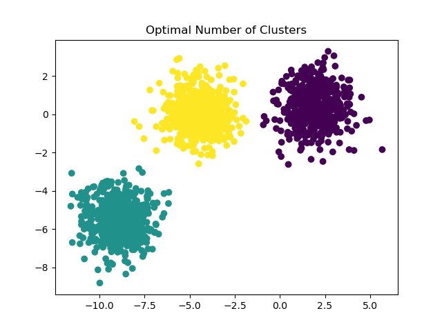
Possible solutions#
For an example on how to find a correct number of blobs, see
Selecting the number of clusters with silhouette analysis on KMeans clustering.
In this case it suffices to set n_clusters=3.
y_pred = KMeans(n_clusters=3, **common_params).fit_predict(X)
plt.scatter(X[:, 0], X[:, 1], c=y_pred)
plt.title("Optimal Number of Clusters")
plt.show()
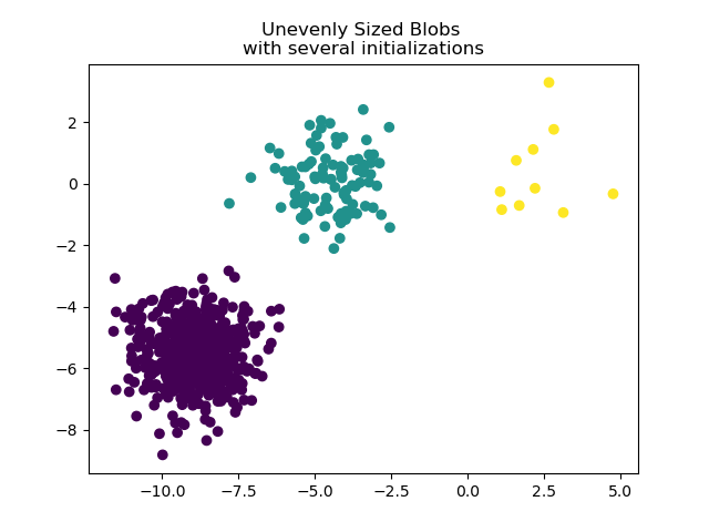
To deal with unevenly sized blobs one can increase the number of random
initializations. In this case we set n_init=10 to avoid finding a
sub-optimal local minimum. For more details see Clustering sparse data with k-means.
y_pred = KMeans(n_clusters=3, n_init=10, random_state=random_state).fit_predict(
    X_filtered
)
plt.scatter(X_filtered[:, 0], X_filtered[:, 1], c=y_pred)
plt.title("Unevenly Sized Blobs \nwith several initializations")
plt.show()
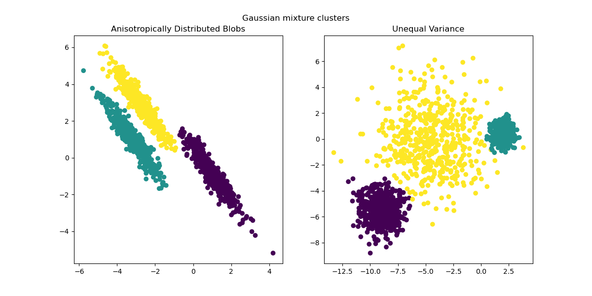
As anisotropic and unequal variances are real limitations of the k-means
algorithm, here we propose instead the use of
GaussianMixture, which also assumes gaussian
clusters but does not impose any constraints on their variances. Notice that
one still has to find the correct number of blobs (see
Gaussian Mixture Model Selection).
For an example on how other clustering methods deal with anisotropic or unequal variance blobs, see the example Comparing different clustering algorithms on toy datasets.
from sklearn.mixture import GaussianMixture

fig, (ax1, ax2) = plt.subplots(nrows=1, ncols=2, figsize=(12, 6))

y_pred = GaussianMixture(n_components=3).fit_predict(X_aniso)
ax1.scatter(X_aniso[:, 0], X_aniso[:, 1], c=y_pred)
ax1.set_title("Anisotropically Distributed Blobs")

y_pred = GaussianMixture(n_components=3).fit_predict(X_varied)
ax2.scatter(X_varied[:, 0], X_varied[:, 1], c=y_pred)
ax2.set_title("Unequal Variance")

plt.suptitle("Gaussian mixture clusters").set_y(0.95)
plt.show()
Final remarks#
In high-dimensional spaces, Euclidean distances tend to become inflated (not shown in this example). Running a dimensionality reduction algorithm prior to k-means clustering can alleviate this problem and speed up the computations (see the example Clustering text documents using k-means).
In the case where clusters are known to be isotropic, have similar variance and are not too sparse, the k-means algorithm is quite effective and is one of the fastest clustering algorithms available. This advantage is lost if one has to restart it several times to avoid convergence to a local minimum.
Total running time of the script: (0 minutes 0.968 seconds)
Related examples
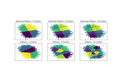
Bisecting K-Means and Regular K-Means Performance Comparison
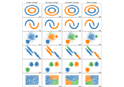
Comparing different hierarchical linkage methods on toy datasets
A demo of K-Means clustering on the handwritten digits data