Note
Go to the end to download the full example code or to run this example in your browser via JupyterLite or Binder.
Kernel PCA#
This example shows the difference between the Principal Components Analysis
(PCA) and its kernelized version
(KernelPCA).
On the one hand, we show that KernelPCA is able
to find a projection of the data which linearly separates them while it is not the case
with PCA.
Finally, we show that inverting this projection is an approximation with
KernelPCA, while it is exact with
PCA.
# Authors: The scikit-learn developers
# SPDX-License-Identifier: BSD-3-Clause
Projecting data: PCA vs. KernelPCA#
In this section, we show the advantages of using a kernel when projecting data using a Principal Component Analysis (PCA). We create a dataset made of two nested circles.
from sklearn.datasets import make_circles
from sklearn.model_selection import train_test_split

X, y = make_circles(n_samples=1_000, factor=0.3, noise=0.05, random_state=0)
X_train, X_test, y_train, y_test = train_test_split(X, y, stratify=y, random_state=0)
Let’s have a quick first look at the generated dataset.
import matplotlib.pyplot as plt

_, (train_ax, test_ax) = plt.subplots(ncols=2, sharex=True, sharey=True, figsize=(8, 4))

train_ax.scatter(X_train[:, 0], X_train[:, 1], c=y_train)
train_ax.set_ylabel("Feature #1")
train_ax.set_xlabel("Feature #0")
train_ax.set_title("Training data")

test_ax.scatter(X_test[:, 0], X_test[:, 1], c=y_test)
test_ax.set_xlabel("Feature #0")
_ = test_ax.set_title("Testing data")
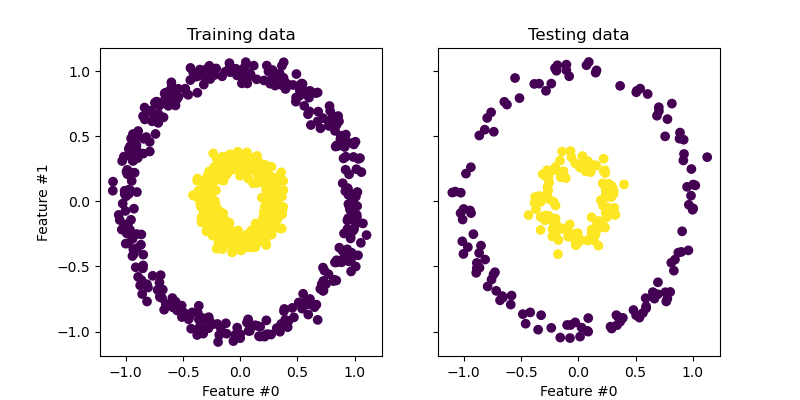
The samples from each class cannot be linearly separated: there is no straight line that can split the samples of the inner set from the outer set.
Now, we will use PCA with and without a kernel to see what is the effect of using such a kernel. The kernel used here is a radial basis function (RBF) kernel.
fig, (orig_data_ax, pca_proj_ax, kernel_pca_proj_ax) = plt.subplots(
    ncols=3, figsize=(14, 4)
)

orig_data_ax.scatter(X_test[:, 0], X_test[:, 1], c=y_test)
orig_data_ax.set_ylabel("Feature #1")
orig_data_ax.set_xlabel("Feature #0")
orig_data_ax.set_title("Testing data")

pca_proj_ax.scatter(X_test_pca[:, 0], X_test_pca[:, 1], c=y_test)
pca_proj_ax.set_ylabel("Principal component #1")
pca_proj_ax.set_xlabel("Principal component #0")
pca_proj_ax.set_title("Projection of testing data\n using PCA")

kernel_pca_proj_ax.scatter(X_test_kernel_pca[:, 0], X_test_kernel_pca[:, 1], c=y_test)
kernel_pca_proj_ax.set_ylabel("Principal component #1")
kernel_pca_proj_ax.set_xlabel("Principal component #0")
_ = kernel_pca_proj_ax.set_title("Projection of testing data\n using KernelPCA")
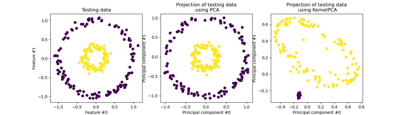
We recall that PCA transforms the data linearly. Intuitively, it means that the coordinate system will be centered, rescaled on each component with respected to its variance and finally be rotated. The obtained data from this transformation is isotropic and can now be projected on its principal components.
Thus, looking at the projection made using PCA (i.e. the middle figure), we see that there is no change regarding the scaling; indeed the data being two concentric circles centered in zero, the original data is already isotropic. However, we can see that the data have been rotated. As a conclusion, we see that such a projection would not help if define a linear classifier to distinguish samples from both classes.
Using a kernel allows to make a non-linear projection. Here, by using an RBF kernel, we expect that the projection will unfold the dataset while keeping approximately preserving the relative distances of pairs of data points that are close to one another in the original space.
We observe such behaviour in the figure on the right: the samples of a given class are closer to each other than the samples from the opposite class, untangling both sample sets. Now, we can use a linear classifier to separate the samples from the two classes.
Projecting into the original feature space#
One particularity to have in mind when using
KernelPCA is related to the reconstruction
(i.e. the back projection in the original feature space). With
PCA, the reconstruction will be exact if
n_components is the same than the number of original features.
This is the case in this example.
We can investigate if we get the original dataset when back projecting with
KernelPCA.
X_reconstructed_pca = pca.inverse_transform(pca.transform(X_test))
X_reconstructed_kernel_pca = kernel_pca.inverse_transform(kernel_pca.transform(X_test))
fig, (orig_data_ax, pca_back_proj_ax, kernel_pca_back_proj_ax) = plt.subplots(
    ncols=3, sharex=True, sharey=True, figsize=(13, 4)
)

orig_data_ax.scatter(X_test[:, 0], X_test[:, 1], c=y_test)
orig_data_ax.set_ylabel("Feature #1")
orig_data_ax.set_xlabel("Feature #0")
orig_data_ax.set_title("Original test data")

pca_back_proj_ax.scatter(X_reconstructed_pca[:, 0], X_reconstructed_pca[:, 1], c=y_test)
pca_back_proj_ax.set_xlabel("Feature #0")
pca_back_proj_ax.set_title("Reconstruction via PCA")

kernel_pca_back_proj_ax.scatter(
    X_reconstructed_kernel_pca[:, 0], X_reconstructed_kernel_pca[:, 1], c=y_test
)
kernel_pca_back_proj_ax.set_xlabel("Feature #0")
_ = kernel_pca_back_proj_ax.set_title("Reconstruction via KernelPCA")
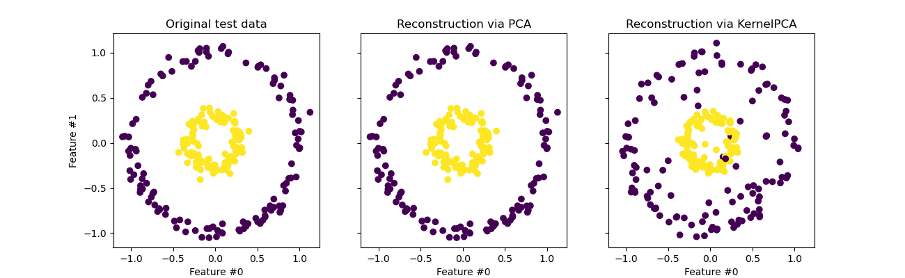
While we see a perfect reconstruction with
PCA we observe a different result for
KernelPCA.
Indeed, inverse_transform cannot
rely on an analytical back-projection and thus an exact reconstruction.
Instead, a KernelRidge is internally trained
to learn a mapping from the kernalized PCA basis to the original feature
space. This method therefore comes with an approximation introducing small
differences when back projecting in the original feature space.
To improve the reconstruction using
inverse_transform, one can tune
alpha in KernelPCA, the regularization term
which controls the reliance on the training data during the training of
the mapping.
Total running time of the script: (0 minutes 0.381 seconds)
Related examples
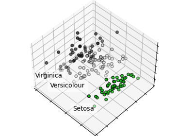
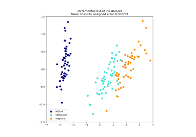
Principal Component Analysis (PCA) on Iris Dataset