Note

Go to the end to download the full example code. or to run this example in your browser via JupyterLite or Binder

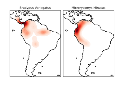
Species distribution modeling#

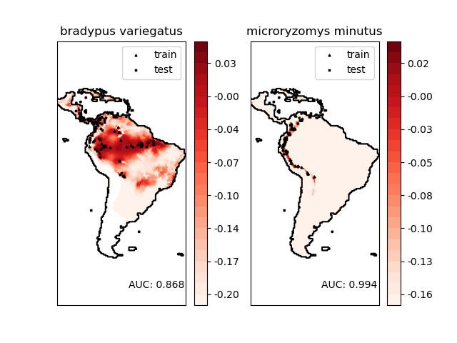
Modeling species’ geographic distributions is an important problem in conservation biology. In this example, we model the geographic distribution of two South American mammals given past observations and 14 environmental variables. Since we have only positive examples (there are no unsuccessful observations), we cast this problem as a density estimation problem and use the OneClassSVM as our modeling tool. The dataset is provided by Phillips et. al. (2006). If available, the example uses basemap to plot the coast lines and national boundaries of South America.

The two species are:

Bradypus variegatus, the brown-throated sloth.
Microryzomys minutus, also known as the forest small rice rat, a rodent that lives in Peru, Colombia, Ecuador, Peru, and Venezuela.

References#

“Maximum entropy modeling of species geographic distributions” S. J. Phillips, R. P. Anderson, R. E. Schapire - Ecological Modelling, 190:231-259, 2006.

bradypus variegatus, microryzomys minutus

________________________________________________________________________________
Modeling distribution of species 'bradypus variegatus'
 - fit OneClassSVM ... done.
 - plot coastlines from coverage
 - predict species distribution

 Area under the ROC curve : 0.868443
________________________________________________________________________________
Modeling distribution of species 'microryzomys minutus'
 - fit OneClassSVM ... done.
 - plot coastlines from coverage
 - predict species distribution

 Area under the ROC curve : 0.993919

time elapsed: 7.03s

# Authors: The scikit-learn developers
# SPDX-License-Identifier: BSD-3-Clause

from time import time

import matplotlib.pyplot as plt
import numpy as np

from sklearn import metrics, svm
from sklearn.datasets import fetch_species_distributions
from sklearn.utils import Bunch

# if basemap is available, we'll use it.
# otherwise, we'll improvise later...
try:
    from mpl_toolkits.basemap import Basemap

    basemap = True
except ImportError:
    basemap = False


def construct_grids(batch):
    """Construct the map grid from the batch object

    Parameters
    ----------
    batch : Batch object
        The object returned by :func:`fetch_species_distributions`

    Returns
    -------
    (xgrid, ygrid) : 1-D arrays
        The grid corresponding to the values in batch.coverages
    """
    # x,y coordinates for corner cells
    xmin = batch.x_left_lower_corner + batch.grid_size
    xmax = xmin + (batch.Nx * batch.grid_size)
    ymin = batch.y_left_lower_corner + batch.grid_size
    ymax = ymin + (batch.Ny * batch.grid_size)

    # x coordinates of the grid cells
    xgrid = np.arange(xmin, xmax, batch.grid_size)
    # y coordinates of the grid cells
    ygrid = np.arange(ymin, ymax, batch.grid_size)

    return (xgrid, ygrid)


def create_species_bunch(species_name, train, test, coverages, xgrid, ygrid):
    """Create a bunch with information about a particular organism

    This will use the test/train record arrays to extract the
    data specific to the given species name.
    """
    bunch = Bunch(name=" ".join(species_name.split("_")[:2]))
    species_name = species_name.encode("ascii")
    points = dict(test=test, train=train)

    for label, pts in points.items():
        # choose points associated with the desired species
        pts = pts[pts["species"] == species_name]
        bunch["pts_%s" % label] = pts

        # determine coverage values for each of the training & testing points
        ix = np.searchsorted(xgrid, pts["dd long"])
        iy = np.searchsorted(ygrid, pts["dd lat"])
        bunch["cov_%s" % label] = coverages[:, -iy, ix].T

    return bunch


def plot_species_distribution(
    species=("bradypus_variegatus_0", "microryzomys_minutus_0")
):
    """
    Plot the species distribution.
    """
    if len(species) > 2:
        print(
            "Note: when more than two species are provided,"
            " only the first two will be used"
        )

    t0 = time()

    # Load the compressed data
    data = fetch_species_distributions()

    # Set up the data grid
    xgrid, ygrid = construct_grids(data)

    # The grid in x,y coordinates
    X, Y = np.meshgrid(xgrid, ygrid[::-1])

    # create a bunch for each species
    BV_bunch = create_species_bunch(
        species[0], data.train, data.test, data.coverages, xgrid, ygrid
    )
    MM_bunch = create_species_bunch(
        species[1], data.train, data.test, data.coverages, xgrid, ygrid
    )

    # background points (grid coordinates) for evaluation
    np.random.seed(13)
    background_points = np.c_[
        np.random.randint(low=0, high=data.Ny, size=10000),
        np.random.randint(low=0, high=data.Nx, size=10000),
    ].T

    # We'll make use of the fact that coverages[6] has measurements at all
    # land points.  This will help us decide between land and water.
    land_reference = data.coverages[6]

    # Fit, predict, and plot for each species.
    for i, species in enumerate([BV_bunch, MM_bunch]):
        print("_" * 80)
        print("Modeling distribution of species '%s'" % species.name)

        # Standardize features
        mean = species.cov_train.mean(axis=0)
        std = species.cov_train.std(axis=0)
        train_cover_std = (species.cov_train - mean) / std

        # Fit OneClassSVM
        print(" - fit OneClassSVM ... ", end="")
        clf = svm.OneClassSVM(nu=0.1, kernel="rbf", gamma=0.5)
        clf.fit(train_cover_std)
        print("done.")

        # Plot map of South America
        plt.subplot(1, 2, i + 1)
        if basemap:
            print(" - plot coastlines using basemap")
            m = Basemap(
                projection="cyl",
                llcrnrlat=Y.min(),
                urcrnrlat=Y.max(),
                llcrnrlon=X.min(),
                urcrnrlon=X.max(),
                resolution="c",
            )
            m.drawcoastlines()
            m.drawcountries()
        else:
            print(" - plot coastlines from coverage")
            plt.contour(
                X, Y, land_reference, levels=[-9998], colors="k", linestyles="solid"
            )
            plt.xticks([])
            plt.yticks([])

        print(" - predict species distribution")

        # Predict species distribution using the training data
        Z = np.ones((data.Ny, data.Nx), dtype=np.float64)

        # We'll predict only for the land points.
        idx = np.where(land_reference > -9999)
        coverages_land = data.coverages[:, idx[0], idx[1]].T

        pred = clf.decision_function((coverages_land - mean) / std)
        Z *= pred.min()
        Z[idx[0], idx[1]] = pred

        levels = np.linspace(Z.min(), Z.max(), 25)
        Z[land_reference == -9999] = -9999

        # plot contours of the prediction
        plt.contourf(X, Y, Z, levels=levels, cmap=plt.cm.Reds)
        plt.colorbar(format="%.2f")

        # scatter training/testing points
        plt.scatter(
            species.pts_train["dd long"],
            species.pts_train["dd lat"],
            s=2**2,
            c="black",
            marker="^",
            label="train",
        )
        plt.scatter(
            species.pts_test["dd long"],
            species.pts_test["dd lat"],
            s=2**2,
            c="black",
            marker="x",
            label="test",
        )
        plt.legend()
        plt.title(species.name)
        plt.axis("equal")

        # Compute AUC with regards to background points
        pred_background = Z[background_points[0], background_points[1]]
        pred_test = clf.decision_function((species.cov_test - mean) / std)
        scores = np.r_[pred_test, pred_background]
        y = np.r_[np.ones(pred_test.shape), np.zeros(pred_background.shape)]
        fpr, tpr, thresholds = metrics.roc_curve(y, scores)
        roc_auc = metrics.auc(fpr, tpr)
        plt.text(-35, -70, "AUC: %.3f" % roc_auc, ha="right")
        print("\n Area under the ROC curve : %f" % roc_auc)

    print("\ntime elapsed: %.2fs" % (time() - t0))


plot_species_distribution()
plt.show()