Note
Go to the end to download the full example code or to run this example in your browser via JupyterLite or Binder.
Multiclass Receiver Operating Characteristic (ROC)#
This example describes the use of the Receiver Operating Characteristic (ROC) metric to evaluate the quality of multiclass classifiers.
ROC curves typically feature true positive rate (TPR) on the Y axis, and false positive rate (FPR) on the X axis. This means that the top left corner of the plot is the “ideal” point - a FPR of zero, and a TPR of one. This is not very realistic, but it does mean that a larger area under the curve (AUC) is usually better. The “steepness” of ROC curves is also important, since it is ideal to maximize the TPR while minimizing the FPR.
ROC curves are typically used in binary classification, where the TPR and FPR can be defined unambiguously. In the case of multiclass classification, a notion of TPR or FPR is obtained only after binarizing the output. This can be done in 2 different ways:
the One-vs-Rest scheme compares each class against all the others (assumed as one);
the One-vs-One scheme compares every unique pairwise combination of classes.
In this example we explore both schemes and demo the concepts of micro and macro averaging as different ways of summarizing the information of the multiclass ROC curves.
Note
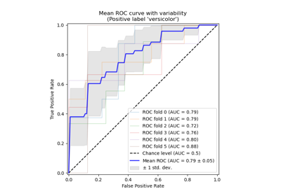
See Receiver Operating Characteristic (ROC) with cross validation for an extension of the present example estimating the variance of the ROC curves and their respective AUC.
# Authors: The scikit-learn developers
# SPDX-License-Identifier: BSD-3-Clause
Load and prepare data#
We import the Iris plants dataset which contains 3 classes, each one corresponding to a type of iris plant. One class is linearly separable from the other 2; the latter are not linearly separable from each other.
Here we binarize the output and add noisy features to make the problem harder.
import numpy as np

from sklearn.datasets import load_iris
from sklearn.model_selection import train_test_split

iris = load_iris()
target_names = iris.target_names
X, y = iris.data, iris.target
y = iris.target_names[y]

random_state = np.random.RandomState(0)
n_samples, n_features = X.shape
n_classes = len(np.unique(y))
X = np.concatenate([X, random_state.randn(n_samples, 200 * n_features)], axis=1)
(
    X_train,
    X_test,
    y_train,
    y_test,
) = train_test_split(X, y, test_size=0.5, stratify=y, random_state=0)
We train a LogisticRegression model which can
naturally handle multiclass problems, thanks to the use of the multinomial
formulation.
from sklearn.linear_model import LogisticRegression

classifier = LogisticRegression()
y_score = classifier.fit(X_train, y_train).predict_proba(X_test)
One-vs-Rest multiclass ROC#
The One-vs-the-Rest (OvR) multiclass strategy, also known as one-vs-all,
consists in computing a ROC curve per each of the n_classes. In each step, a
given class is regarded as the positive class and the remaining classes are
regarded as the negative class as a bulk.
Note
One should not confuse the OvR strategy used for the evaluation
of multiclass classifiers with the OvR strategy used to train a
multiclass classifier by fitting a set of binary classifiers (for instance
via the OneVsRestClassifier meta-estimator).
The OvR ROC evaluation can be used to scrutinize any kind of classification
models irrespectively of how they were trained (see Multiclass and multioutput algorithms).
In this section we use a LabelBinarizer to
binarize the target by one-hot-encoding in a OvR fashion. This means that the
target of shape (n_samples,) is mapped to a target of shape (n_samples,
n_classes).
from sklearn.preprocessing import LabelBinarizer

label_binarizer = LabelBinarizer().fit(y_train)
y_onehot_test = label_binarizer.transform(y_test)
y_onehot_test.shape  # (n_samples, n_classes)
(75, 3)
We can as well easily check the encoding of a specific class:
label_binarizer.transform(["virginica"])
array([[0, 0, 1]])
ROC curve showing a specific class#
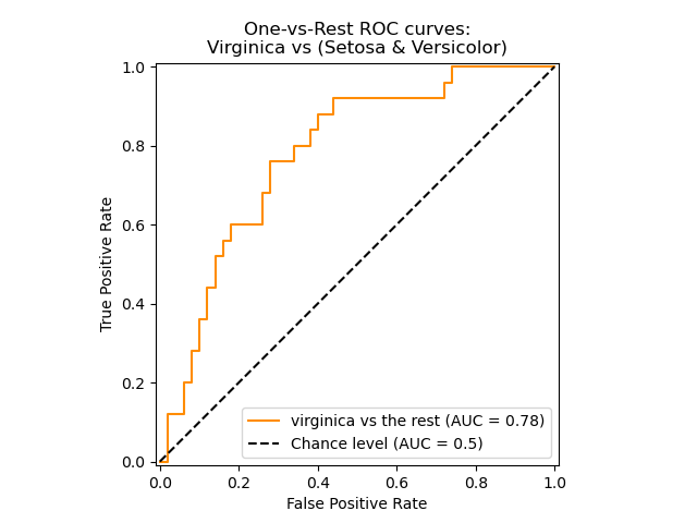
In the following plot we show the resulting ROC curve when regarding the iris
flowers as either “virginica” (class_id=2) or “non-virginica” (the rest).
class_of_interest = "virginica"
class_id = np.flatnonzero(label_binarizer.classes_ == class_of_interest)[0]
class_id
np.int64(2)
import matplotlib.pyplot as plt

from sklearn.metrics import RocCurveDisplay

display = RocCurveDisplay.from_predictions(
    y_onehot_test[:, class_id],
    y_score[:, class_id],
    name=f"{class_of_interest} vs the rest",
    curve_kwargs=dict(color="darkorange"),
    plot_chance_level=True,
    despine=True,
)
_ = display.ax_.set(
    xlabel="False Positive Rate",
    ylabel="True Positive Rate",
    title="One-vs-Rest ROC curves:\nVirginica vs (Setosa & Versicolor)",
)
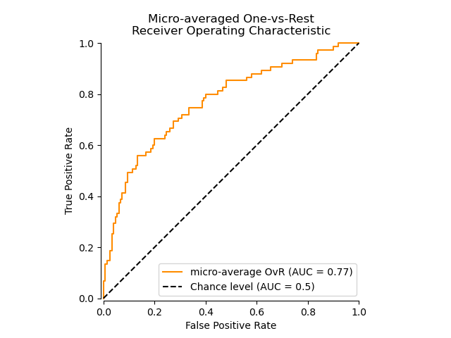
ROC curve using micro-averaged OvR#
Micro-averaging aggregates the contributions from all the classes (using
numpy.ravel) to compute the average metrics as follows:
\(TPR=\frac{\sum_{c}TP_c}{\sum_{c}(TP_c + FN_c)}\) ;
\(FPR=\frac{\sum_{c}FP_c}{\sum_{c}(FP_c + TN_c)}\) .
We can briefly demo the effect of numpy.ravel:
print(f"y_score:\n{y_score[0:2, :]}")
print()
print(f"y_score.ravel():\n{y_score[0:2, :].ravel()}")
y_score:
[[0.38 0.05 0.57]
 [0.07 0.28 0.65]]

y_score.ravel():
[0.38 0.05 0.57 0.07 0.28 0.65]
In a multi-class classification setup with highly imbalanced classes, micro-averaging is preferable over macro-averaging. In such cases, one can alternatively use a weighted macro-averaging, not demonstrated here.
display = RocCurveDisplay.from_predictions(
    y_onehot_test.ravel(),
    y_score.ravel(),
    name="micro-average OvR",
    curve_kwargs=dict(color="darkorange"),
    plot_chance_level=True,
    despine=True,
)
_ = display.ax_.set(
    xlabel="False Positive Rate",
    ylabel="True Positive Rate",
    title="Micro-averaged One-vs-Rest\nReceiver Operating Characteristic",
)
In the case where the main interest is not the plot but the ROC-AUC score
itself, we can reproduce the value shown in the plot using
roc_auc_score.
from sklearn.metrics import roc_auc_score

micro_roc_auc_ovr = roc_auc_score(
    y_test,
    y_score,
    multi_class="ovr",
    average="micro",
)

print(f"Micro-averaged One-vs-Rest ROC AUC score:\n{micro_roc_auc_ovr:.2f}")
Micro-averaged One-vs-Rest ROC AUC score:
0.77
This is equivalent to computing the ROC curve with
roc_curve and then the area under the curve with
auc for the raveled true and predicted classes.
from sklearn.metrics import auc, roc_curve

# store the fpr, tpr, and roc_auc for all averaging strategies
fpr, tpr, roc_auc = dict(), dict(), dict()
# Compute micro-average ROC curve and ROC area
fpr["micro"], tpr["micro"], _ = roc_curve(y_onehot_test.ravel(), y_score.ravel())
roc_auc["micro"] = auc(fpr["micro"], tpr["micro"])

print(f"Micro-averaged One-vs-Rest ROC AUC score:\n{roc_auc['micro']:.2f}")
Micro-averaged One-vs-Rest ROC AUC score:
0.77
Note
By default, the computation of the ROC curve adds a single point at the maximal false positive rate by using linear interpolation and the McClish correction [Analyzing a portion of the ROC curve Med Decis Making. 1989 Jul-Sep; 9(3):190-5.].
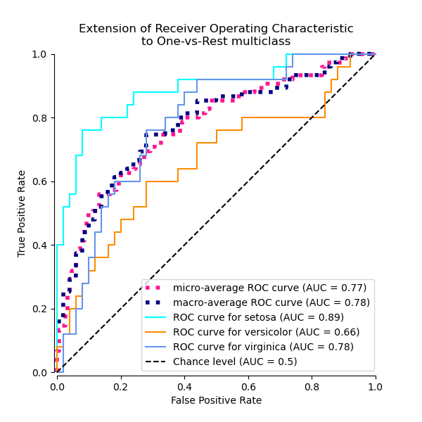
ROC curve using the OvR macro-average#
Obtaining the macro-average requires computing the metric independently for each class and then taking the average over them, hence treating all classes equally a priori. We first aggregate the true/false positive rates per class:
\(TPR=\frac{1}{C}\sum_{c}\frac{TP_c}{TP_c + FN_c}\) ;
\(FPR=\frac{1}{C}\sum_{c}\frac{FP_c}{FP_c + TN_c}\) .
where C is the total number of classes.
for i in range(n_classes):
    fpr[i], tpr[i], _ = roc_curve(y_onehot_test[:, i], y_score[:, i])
    roc_auc[i] = auc(fpr[i], tpr[i])

fpr_grid = np.linspace(0.0, 1.0, 1000)

# Interpolate all ROC curves at these points
mean_tpr = np.zeros_like(fpr_grid)

for i in range(n_classes):
    mean_tpr += np.interp(fpr_grid, fpr[i], tpr[i])  # linear interpolation

# Average it and compute AUC
mean_tpr /= n_classes

fpr["macro"] = fpr_grid
tpr["macro"] = mean_tpr
roc_auc["macro"] = auc(fpr["macro"], tpr["macro"])

print(f"Macro-averaged One-vs-Rest ROC AUC score:\n{roc_auc['macro']:.2f}")
Macro-averaged One-vs-Rest ROC AUC score:
0.78
This computation is equivalent to simply calling
macro_roc_auc_ovr = roc_auc_score(
    y_test,
    y_score,
    multi_class="ovr",
    average="macro",
)

print(f"Macro-averaged One-vs-Rest ROC AUC score:\n{macro_roc_auc_ovr:.2f}")
Macro-averaged One-vs-Rest ROC AUC score:
0.78
Plot all OvR ROC curves together#
from itertools import cycle

fig, ax = plt.subplots(figsize=(6, 6))

plt.plot(
    fpr["micro"],
    tpr["micro"],
    label=f"micro-average ROC curve (AUC = {roc_auc['micro']:.2f})",
    color="deeppink",
    linestyle=":",
    linewidth=4,
)

plt.plot(
    fpr["macro"],
    tpr["macro"],
    label=f"macro-average ROC curve (AUC = {roc_auc['macro']:.2f})",
    color="navy",
    linestyle=":",
    linewidth=4,
)

colors = cycle(["aqua", "darkorange", "cornflowerblue"])
for class_id, color in zip(range(n_classes), colors):
    RocCurveDisplay.from_predictions(
        y_onehot_test[:, class_id],
        y_score[:, class_id],
        name=f"ROC curve for {target_names[class_id]}",
        curve_kwargs=dict(color=color),
        ax=ax,
        plot_chance_level=(class_id == 2),
        despine=True,
    )

_ = ax.set(
    xlabel="False Positive Rate",
    ylabel="True Positive Rate",
    title="Extension of Receiver Operating Characteristic\nto One-vs-Rest multiclass",
)
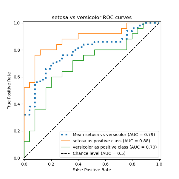
One-vs-One multiclass ROC#
The One-vs-One (OvO) multiclass strategy consists in fitting one classifier
per class pair. Since it requires to train n_classes * (n_classes - 1) / 2
classifiers, this method is usually slower than One-vs-Rest due to its
O(n_classes ^2) complexity.
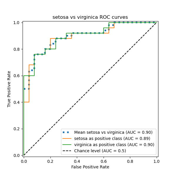
In this section, we demonstrate the macro-averaged AUC using the OvO scheme for the 3 possible combinations in the Iris plants dataset: “setosa” vs “versicolor”, “versicolor” vs “virginica” and “virginica” vs “setosa”. Notice that micro-averaging is not defined for the OvO scheme.
ROC curve using the OvO macro-average#
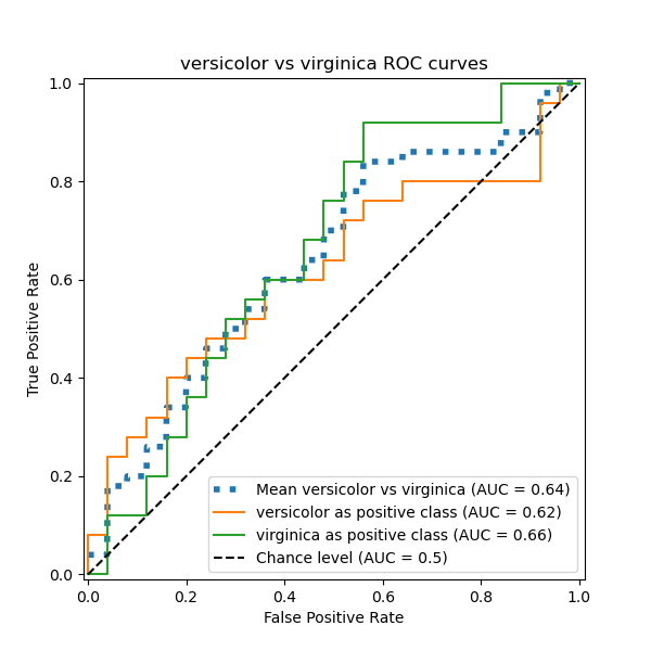
In the OvO scheme, the first step is to identify all possible unique combinations of pairs. The computation of scores is done by treating one of the elements in a given pair as the positive class and the other element as the negative class, then re-computing the score by inversing the roles and taking the mean of both scores.
from itertools import combinations

pair_list = list(combinations(np.unique(y), 2))
print(pair_list)
[(np.str_('setosa'), np.str_('versicolor')), (np.str_('setosa'), np.str_('virginica')), (np.str_('versicolor'), np.str_('virginica'))]
pair_scores = []
mean_tpr = dict()

for ix, (label_a, label_b) in enumerate(pair_list):
    a_mask = y_test == label_a
    b_mask = y_test == label_b
    ab_mask = np.logical_or(a_mask, b_mask)

    a_true = a_mask[ab_mask]
    b_true = b_mask[ab_mask]

    idx_a = np.flatnonzero(label_binarizer.classes_ == label_a)[0]
    idx_b = np.flatnonzero(label_binarizer.classes_ == label_b)[0]

    fpr_a, tpr_a, _ = roc_curve(a_true, y_score[ab_mask, idx_a])
    fpr_b, tpr_b, _ = roc_curve(b_true, y_score[ab_mask, idx_b])

    mean_tpr[ix] = np.zeros_like(fpr_grid)
    mean_tpr[ix] += np.interp(fpr_grid, fpr_a, tpr_a)
    mean_tpr[ix] += np.interp(fpr_grid, fpr_b, tpr_b)
    mean_tpr[ix] /= 2
    mean_score = auc(fpr_grid, mean_tpr[ix])
    pair_scores.append(mean_score)

    fig, ax = plt.subplots(figsize=(6, 6))
    plt.plot(
        fpr_grid,
        mean_tpr[ix],
        label=f"Mean {label_a} vs {label_b} (AUC = {mean_score:.2f})",
        linestyle=":",
        linewidth=4,
    )
    RocCurveDisplay.from_predictions(
        a_true,
        y_score[ab_mask, idx_a],
        ax=ax,
        name=f"{label_a} as positive class",
    )
    RocCurveDisplay.from_predictions(
        b_true,
        y_score[ab_mask, idx_b],
        ax=ax,
        name=f"{label_b} as positive class",
        plot_chance_level=True,
        despine=True,
    )
    ax.set(
        xlabel="False Positive Rate",
        ylabel="True Positive Rate",
        title=f"{target_names[idx_a]} vs {label_b} ROC curves",
    )

print(f"Macro-averaged One-vs-One ROC AUC score:\n{np.average(pair_scores):.2f}")
Macro-averaged One-vs-One ROC AUC score:
0.78
One can also assert that the macro-average we computed “by hand” is equivalent
to the implemented average="macro" option of the
roc_auc_score function.
macro_roc_auc_ovo = roc_auc_score(
    y_test,
    y_score,
    multi_class="ovo",
    average="macro",
)

print(f"Macro-averaged One-vs-One ROC AUC score:\n{macro_roc_auc_ovo:.2f}")
Macro-averaged One-vs-One ROC AUC score:
0.78
Plot all OvO ROC curves together#
ovo_tpr = np.zeros_like(fpr_grid)

fig, ax = plt.subplots(figsize=(6, 6))
for ix, (label_a, label_b) in enumerate(pair_list):
    ovo_tpr += mean_tpr[ix]
    ax.plot(
        fpr_grid,
        mean_tpr[ix],
        label=f"Mean {label_a} vs {label_b} (AUC = {pair_scores[ix]:.2f})",
    )

ovo_tpr /= sum(1 for pair in enumerate(pair_list))

ax.plot(
    fpr_grid,
    ovo_tpr,
    label=f"One-vs-One macro-average (AUC = {macro_roc_auc_ovo:.2f})",
    linestyle=":",
    linewidth=4,
)
ax.plot([0, 1], [0, 1], "k--", label="Chance level (AUC = 0.5)")
_ = ax.set(
    xlabel="False Positive Rate",
    ylabel="True Positive Rate",
    title="Extension of Receiver Operating Characteristic\nto One-vs-One multiclass",
    aspect="equal",
    xlim=(-0.01, 1.01),
    ylim=(-0.01, 1.01),
)
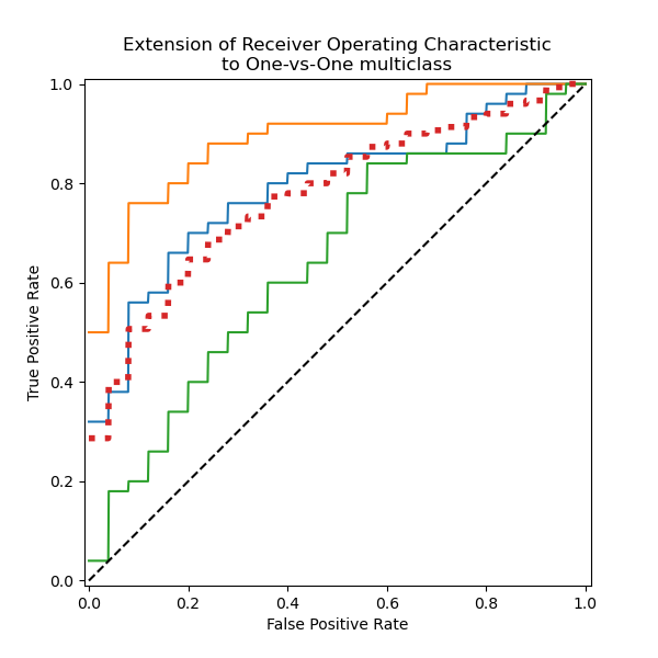
We confirm that the classes “versicolor” and “virginica” are not well identified by a linear classifier. Notice that the “virginica”-vs-the-rest ROC-AUC score (0.77) is between the OvO ROC-AUC scores for “versicolor” vs “virginica” (0.64) and “setosa” vs “virginica” (0.90). Indeed, the OvO strategy gives additional information on the confusion between a pair of classes, at the expense of computational cost when the number of classes is large.
The OvO strategy is recommended if the user is mainly interested in correctly identifying a particular class or subset of classes, whereas evaluating the global performance of a classifier can still be summarized via a given averaging strategy.
When dealing with imbalanced datasets, choosing the appropriate metric based on the business context or problem you are addressing is crucial. It is also essential to select an appropriate averaging method (micro vs. macro) depending on the desired outcome:
Micro-averaging aggregates metrics across all instances, treating each individual instance equally, regardless of its class. This approach is useful when evaluating overall performance, but note that it can be dominated by the majority class in imbalanced datasets.
Macro-averaging calculates metrics for each class independently and then averages them, giving equal weight to each class. This is particularly useful when you want under-represented classes to be considered as important as highly populated classes.
Total running time of the script: (0 minutes 0.808 seconds)
Related examples
Receiver Operating Characteristic (ROC) with cross validation