Partial Dependence and Individual Conditional Expectation Plots

Partial dependence plots show the dependence between the target function [2] and a set of features of interest, marginalizing over the values of all other features (the complement features). Due to the limits of human perception, the size of the set of features of interest must be small (usually, one or two) thus they are usually chosen among the most important features.

Similarly, an individual conditional expectation (ICE) plot [3] shows the dependence between the target function and a feature of interest. However, unlike partial dependence plots, which show the average effect of the features of interest, ICE plots visualize the dependence of the prediction on a feature for each sample separately, with one line per sample. Only one feature of interest is supported for ICE plots.

This example shows how to obtain partial dependence and ICE plots from a MLPRegressor and a HistGradientBoostingRegressor trained on the bike sharing dataset. The example is inspired by [1].

[1]

Molnar, Christoph. “Interpretable machine learning. A Guide for Making Black Box Models Explainable”, 2019.

[2]

For classification you can think of it as the regression score before the link function.

[3]

Goldstein, A., Kapelner, A., Bleich, J., and Pitkin, E. (2015). “Peeking Inside the Black Box: Visualizing Statistical Learning With Plots of Individual Conditional Expectation”. Journal of Computational and Graphical Statistics, 24(1): 44-65

# Authors: The scikit-learn developers
# SPDX-License-Identifier: BSD-3-Clause

Bike sharing dataset preprocessing

We will use the bike sharing dataset. The goal is to predict the number of bike rentals using weather and season data as well as the datetime information.

from sklearn.datasets import fetch_openml

bikes = fetch_openml("Bike_Sharing_Demand", version=2, as_frame=True)
# Make an explicit copy to avoid "SettingWithCopyWarning" from pandas
X, y = bikes.data.copy(), bikes.target

# We use only a subset of the data to speed up the example.
X = X.iloc[::5, :]
y = y[::5]

The feature "weather" has a particularity: the category "heavy_rain" is a rare category.

X["weather"].value_counts()

weather
clear         2284
misty          904
rain           287
heavy_rain       1
Name: count, dtype: int64

Because of this rare category, we collapse it into "rain".

X["weather"] = (
    X["weather"]
    .astype(object)
    .replace(to_replace="heavy_rain", value="rain")
    .astype("category")
)

We now have a closer look at the "year" feature:

X["year"].value_counts()

year
1    1747
0    1729
Name: count, dtype: int64

We see that we have data from two years. We use the first year to train the model and the second year to test the model.

mask_training = X["year"] == 0.0
X = X.drop(columns=["year"])
X_train, y_train = X[mask_training], y[mask_training]
X_test, y_test = X[~mask_training], y[~mask_training]

We can check the dataset information to see that we have heterogeneous data types. We have to preprocess the different columns accordingly.

X_train.info()

<class 'pandas.core.frame.DataFrame'>
Index: 1729 entries, 0 to 8640
Data columns (total 11 columns):
 #   Column      Non-Null Count  Dtype
---  ------      --------------  -----
 0   season      1729 non-null   category
 1   month       1729 non-null   int64
 2   hour        1729 non-null   int64
 3   holiday     1729 non-null   category
 4   weekday     1729 non-null   int64
 5   workingday  1729 non-null   category
 6   weather     1729 non-null   category
 7   temp        1729 non-null   float64
 8   feel_temp   1729 non-null   float64
 9   humidity    1729 non-null   float64
 10  windspeed   1729 non-null   float64
dtypes: category(4), float64(4), int64(3)
memory usage: 115.4 KB

From the previous information, we will consider the category columns as nominal categorical features. In addition, we will consider the date and time information as categorical features as well.

We manually define the columns containing numerical and categorical features.

numerical_features = [
    "temp",
    "feel_temp",
    "humidity",
    "windspeed",
]
categorical_features = X_train.columns.drop(numerical_features)

Before we go into the details regarding the preprocessing of the different machine learning pipelines, we will try to get some additional intuition regarding the dataset that will be helpful to understand the model’s statistical performance and results of the partial dependence analysis.

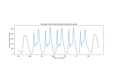
We plot the average number of bike rentals by grouping the data by season and by year.

from itertools import product

import matplotlib.pyplot as plt
import numpy as np

days = ("Sun", "Mon", "Tue", "Wed", "Thu", "Fri", "Sat")
hours = tuple(range(24))
xticklabels = [f"{day}\n{hour}:00" for day, hour in product(days, hours)]
xtick_start, xtick_period = 6, 12

fig, axs = plt.subplots(nrows=2, figsize=(8, 6), sharey=True, sharex=True)
average_bike_rentals = bikes.frame.groupby(
    ["year", "season", "weekday", "hour"], observed=True
).mean(numeric_only=True)["count"]
for ax, (idx, df) in zip(axs, average_bike_rentals.groupby("year")):
    df.groupby("season", observed=True).plot(ax=ax, legend=True)

    # decorate the plot
    ax.set_xticks(
        np.linspace(
            start=xtick_start,
            stop=len(xticklabels),
            num=len(xticklabels) // xtick_period,
        )
    )
    ax.set_xticklabels(xticklabels[xtick_start::xtick_period])
    ax.set_xlabel("")
    ax.set_ylabel("Average number of bike rentals")
    ax.set_title(
        f"Bike rental for {'2010 (train set)' if idx == 0.0 else '2011 (test set)'}"
    )
    ax.set_ylim(0, 1_000)
    ax.set_xlim(0, len(xticklabels))
    ax.legend(loc=2)

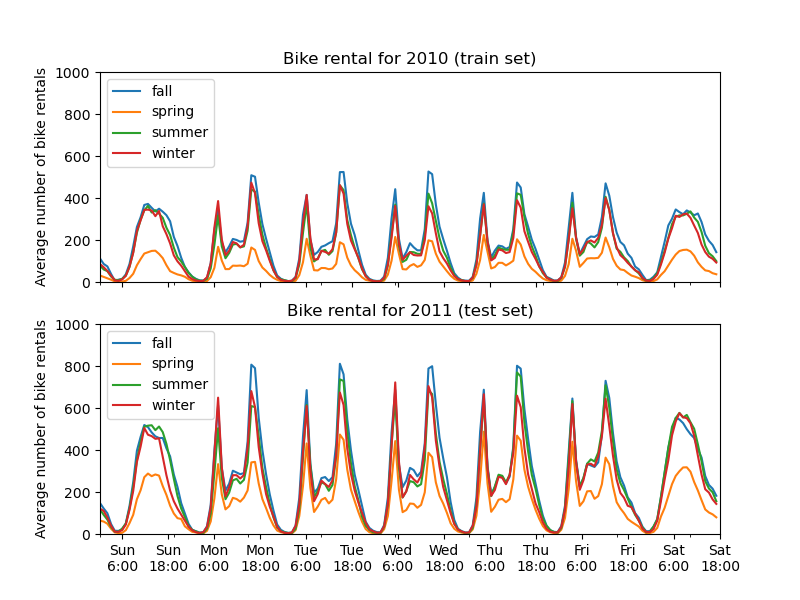
The first striking difference between the train and test set is that the number of bike rentals is higher in the test set. For this reason, it will not be surprising to get a machine learning model that underestimates the number of bike rentals. We also observe that the number of bike rentals is lower during the spring season. In addition, we see that during working days, there is a specific pattern around 6-7 am and 5-6 pm with some peaks of bike rentals. We can keep in mind these different insights and use them to understand the partial dependence plot.

Preprocessor for machine-learning models

Since we later use two different models, a MLPRegressor and a HistGradientBoostingRegressor, we create two different preprocessors, specific for each model.

Preprocessor for the neural network model

We will use a QuantileTransformer to scale the numerical features and encode the categorical features with a OneHotEncoder.

from sklearn.compose import ColumnTransformer
from sklearn.preprocessing import OneHotEncoder, QuantileTransformer

mlp_preprocessor = ColumnTransformer(
    transformers=[
        ("num", QuantileTransformer(n_quantiles=100), numerical_features),
        ("cat", OneHotEncoder(handle_unknown="ignore"), categorical_features),
    ]
)
mlp_preprocessor

ColumnTransformer(transformers=[('num', QuantileTransformer(n_quantiles=100),
                                 ['temp', 'feel_temp', 'humidity',
                                  'windspeed']),
                                ('cat', OneHotEncoder(handle_unknown='ignore'),
                                 Index(['season', 'month', 'hour', 'holiday', 'weekday', 'workingday',
       'weather'],
      dtype='object'))])

In a Jupyter environment, please rerun this cell to show the HTML representation or trust the notebook.
On GitHub, the HTML representation is unable to render, please try loading this page with nbviewer.org.

Preprocessor for the gradient boosting model

For the gradient boosting model, we leave the numerical features as-is and only encode the categorical features using a OrdinalEncoder.

from sklearn.preprocessing import OrdinalEncoder

hgbdt_preprocessor = ColumnTransformer(
    transformers=[
        ("cat", OrdinalEncoder(), categorical_features),
        ("num", "passthrough", numerical_features),
    ],
    sparse_threshold=1,
    verbose_feature_names_out=False,
).set_output(transform="pandas")
hgbdt_preprocessor

ColumnTransformer(sparse_threshold=1,
                  transformers=[('cat', OrdinalEncoder(),
                                 Index(['season', 'month', 'hour', 'holiday', 'weekday', 'workingday',
       'weather'],
      dtype='object')),
                                ('num', 'passthrough',
                                 ['temp', 'feel_temp', 'humidity',
                                  'windspeed'])],
                  verbose_feature_names_out=False)

In a Jupyter environment, please rerun this cell to show the HTML representation or trust the notebook.
On GitHub, the HTML representation is unable to render, please try loading this page with nbviewer.org.

1-way partial dependence with different models

In this section, we will compute 1-way partial dependence with two different machine-learning models: (i) a multi-layer perceptron and (ii) a gradient-boosting model. With these two models, we illustrate how to compute and interpret both partial dependence plot (PDP) for both numerical and categorical features and individual conditional expectation (ICE).

Multi-layer perceptron

Let’s fit a MLPRegressor and compute single-variable partial dependence plots.

from time import time

from sklearn.neural_network import MLPRegressor
from sklearn.pipeline import make_pipeline

print("Training MLPRegressor...")
tic = time()
mlp_model = make_pipeline(
    mlp_preprocessor,
    MLPRegressor(
        hidden_layer_sizes=(30, 15),
        learning_rate_init=0.01,
        early_stopping=True,
        random_state=0,
    ),
)
mlp_model.fit(X_train, y_train)
print(f"done in {time() - tic:.3f}s")
print(f"Test R2 score: {mlp_model.score(X_test, y_test):.2f}")

Training MLPRegressor...
done in 0.787s
Test R2 score: 0.61

We configured a pipeline using the preprocessor that we created specifically for the neural network and tuned the neural network size and learning rate to get a reasonable compromise between training time and predictive performance on a test set.

Importantly, this tabular dataset has very different dynamic ranges for its features. Neural networks tend to be very sensitive to features with varying scales and forgetting to preprocess the numeric feature would lead to a very poor model.

It would be possible to get even higher predictive performance with a larger neural network but the training would also be significantly more expensive.

Note that it is important to check that the model is accurate enough on a test set before plotting the partial dependence since there would be little use in explaining the impact of a given feature on the prediction function of a model with poor predictive performance. In this regard, our MLP model works reasonably well.

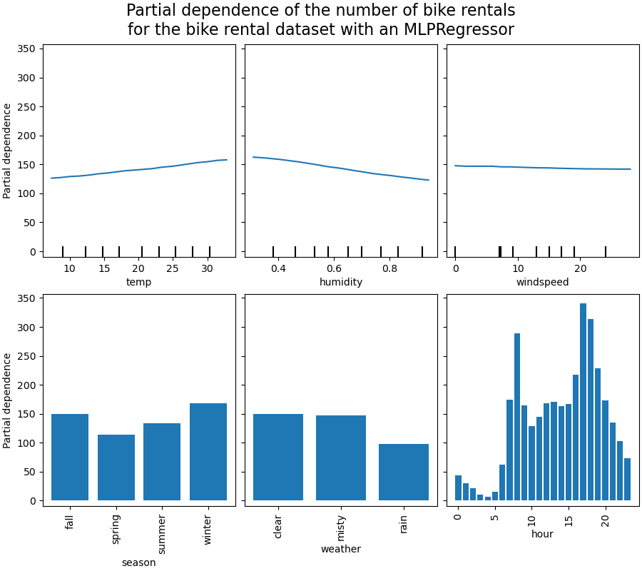
We will plot the averaged partial dependence.

import matplotlib.pyplot as plt

from sklearn.inspection import PartialDependenceDisplay

common_params = {
    "subsample": 50,
    "n_jobs": 2,
    "grid_resolution": 20,
    "random_state": 0,
}

print("Computing partial dependence plots...")
features_info = {
    # features of interest
    "features": ["temp", "humidity", "windspeed", "season", "weather", "hour"],
    # type of partial dependence plot
    "kind": "average",
    # information regarding categorical features
    "categorical_features": categorical_features,
}
tic = time()
_, ax = plt.subplots(ncols=3, nrows=2, figsize=(9, 8), constrained_layout=True)
display = PartialDependenceDisplay.from_estimator(
    mlp_model,
    X_train,
    **features_info,
    ax=ax,
    **common_params,
)
print(f"done in {time() - tic:.3f}s")
_ = display.figure_.suptitle(
    (
        "Partial dependence of the number of bike rentals\n"
        "for the bike rental dataset with an MLPRegressor"
    ),
    fontsize=16,
)

Computing partial dependence plots...
done in 0.678s

Gradient boosting

Let’s now fit a HistGradientBoostingRegressor and compute the partial dependence on the same features. We also use the specific preprocessor we created for this model.

from sklearn.ensemble import HistGradientBoostingRegressor

print("Training HistGradientBoostingRegressor...")
tic = time()
hgbdt_model = make_pipeline(
    hgbdt_preprocessor,
    HistGradientBoostingRegressor(
        categorical_features=categorical_features,
        random_state=0,
        max_iter=50,
    ),
)
hgbdt_model.fit(X_train, y_train)
print(f"done in {time() - tic:.3f}s")
print(f"Test R2 score: {hgbdt_model.score(X_test, y_test):.2f}")

Training HistGradientBoostingRegressor...
done in 0.121s
Test R2 score: 0.62

Here, we used the default hyperparameters for the gradient boosting model without any preprocessing as tree-based models are naturally robust to monotonic transformations of numerical features.

Note that on this tabular dataset, Gradient Boosting Machines are both significantly faster to train and more accurate than neural networks. It is also significantly cheaper to tune their hyperparameters (the defaults tend to work well while this is not often the case for neural networks).

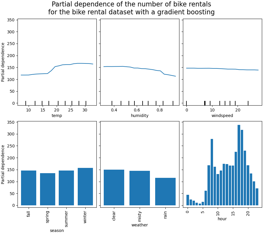
We will plot the partial dependence for some of the numerical and categorical features.

print("Computing partial dependence plots...")
tic = time()
_, ax = plt.subplots(ncols=3, nrows=2, figsize=(9, 8), constrained_layout=True)
display = PartialDependenceDisplay.from_estimator(
    hgbdt_model,
    X_train,
    **features_info,
    ax=ax,
    **common_params,
)
print(f"done in {time() - tic:.3f}s")
_ = display.figure_.suptitle(
    (
        "Partial dependence of the number of bike rentals\n"
        "for the bike rental dataset with a gradient boosting"
    ),
    fontsize=16,
)

Computing partial dependence plots...
done in 1.260s

Analysis of the plots

We will first look at the PDPs for the numerical features. For both models, the general trend of the PDP of the temperature is that the number of bike rentals is increasing with temperature. We can make a similar analysis but with the opposite trend for the humidity features. The number of bike rentals is decreasing when the humidity increases. Finally, we see the same trend for the wind speed feature. The number of bike rentals is decreasing when the wind speed is increasing for both models. We also observe that MLPRegressor has much smoother predictions than HistGradientBoostingRegressor.

Now, we will look at the partial dependence plots for the categorical features.

We observe that the spring season is the lowest bar for the season feature. With the weather feature, the rain category is the lowest bar. Regarding the hour feature, we see two peaks around the 7 am and 6 pm. These findings are in line with the the observations we made earlier on the dataset.

However, it is worth noting that we are creating potential meaningless synthetic samples if features are correlated.

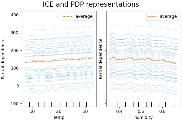
ICE vs. PDP

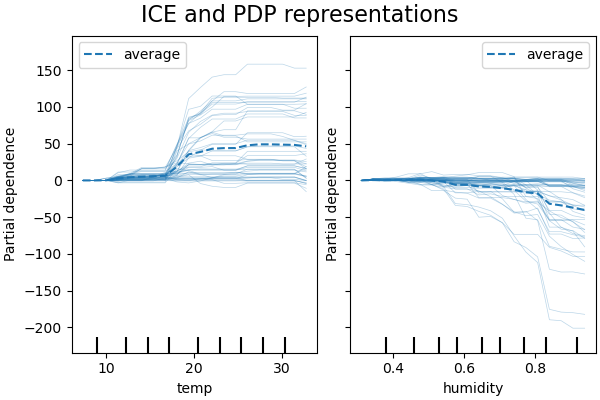
PDP is an average of the marginal effects of the features. We are averaging the response of all samples of the provided set. Thus, some effects could be hidden. In this regard, it is possible to plot each individual response. This representation is called the Individual Effect Plot (ICE). In the plot below, we plot 50 randomly selected ICEs for the temperature and humidity features.

print("Computing partial dependence plots and individual conditional expectation...")
tic = time()
_, ax = plt.subplots(ncols=2, figsize=(6, 4), sharey=True, constrained_layout=True)

features_info = {
    "features": ["temp", "humidity"],
    "kind": "both",
    "centered": True,
}

display = PartialDependenceDisplay.from_estimator(
    hgbdt_model,
    X_train,
    **features_info,
    ax=ax,
    **common_params,
)
print(f"done in {time() - tic:.3f}s")
_ = display.figure_.suptitle("ICE and PDP representations", fontsize=16)

Computing partial dependence plots and individual conditional expectation...
done in 0.584s

We see that the ICE for the temperature feature gives us some additional information: Some of the ICE lines are flat while some others show a decrease of the dependence for temperature above 35 degrees Celsius. We observe a similar pattern for the humidity feature: some of the ICEs lines show a sharp decrease when the humidity is above 80%.

Not all ICE lines are parallel, this indicates that the model finds interactions between features. We can repeat the experiment by constraining the gradient boosting model to not use any interactions between features using the parameter interaction_cst:

from sklearn.base import clone

interaction_cst = [[i] for i in range(X_train.shape[1])]
hgbdt_model_without_interactions = (
    clone(hgbdt_model)
    .set_params(histgradientboostingregressor__interaction_cst=interaction_cst)
    .fit(X_train, y_train)
)
print(f"Test R2 score: {hgbdt_model_without_interactions.score(X_test, y_test):.2f}")

Test R2 score: 0.38

_, ax = plt.subplots(ncols=2, figsize=(6, 4), sharey=True, constrained_layout=True)

features_info["centered"] = False
display = PartialDependenceDisplay.from_estimator(
    hgbdt_model_without_interactions,
    X_train,
    **features_info,
    ax=ax,
    **common_params,
)
_ = display.figure_.suptitle("ICE and PDP representations", fontsize=16)

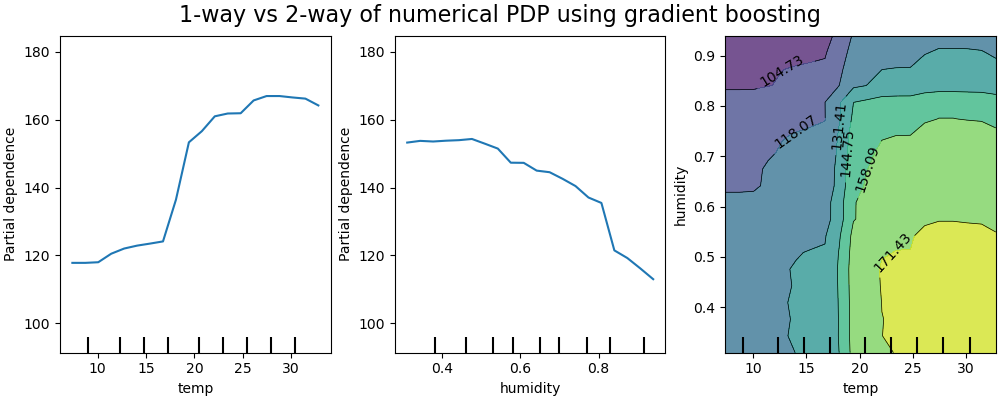
2D interaction plots

PDPs with two features of interest enable us to visualize interactions among them. However, ICEs cannot be plotted in an easy manner and thus interpreted. We will show the representation of available in from_estimator that is a 2D heatmap.

print("Computing partial dependence plots...")
features_info = {
    "features": ["temp", "humidity", ("temp", "humidity")],
    "kind": "average",
}
_, ax = plt.subplots(ncols=3, figsize=(10, 4), constrained_layout=True)
tic = time()
display = PartialDependenceDisplay.from_estimator(
    hgbdt_model,
    X_train,
    **features_info,
    ax=ax,
    **common_params,
)
print(f"done in {time() - tic:.3f}s")
_ = display.figure_.suptitle(
    "1-way vs 2-way of numerical PDP using gradient boosting", fontsize=16
)

Computing partial dependence plots...
done in 8.813s

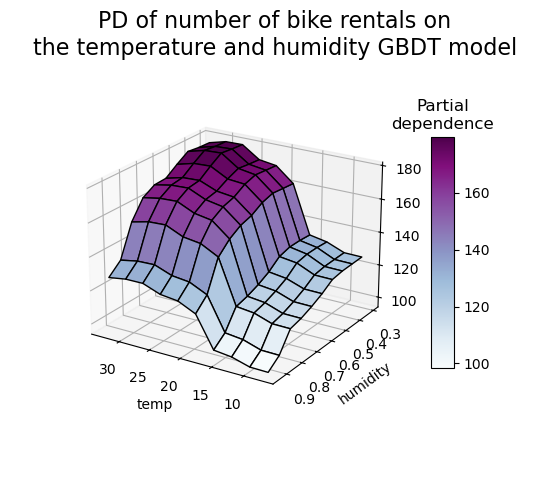
The two-way partial dependence plot shows the dependence of the number of bike rentals on joint values of temperature and humidity. We clearly see an interaction between the two features. For a temperature higher than 20 degrees Celsius, the humidity has a impact on the number of bike rentals that seems independent on the temperature.

On the other hand, for temperatures lower than 20 degrees Celsius, both the temperature and humidity continuously impact the number of bike rentals.

Furthermore, the slope of the of the impact ridge of the 20 degrees Celsius threshold is very dependent on the humidity level: the ridge is steep under dry conditions but much smoother under wetter conditions above 70% of humidity.

We now contrast those results with the same plots computed for the model constrained to learn a prediction function that does not depend on such non-linear feature interactions.

print("Computing partial dependence plots...")
features_info = {
    "features": ["temp", "humidity", ("temp", "humidity")],
    "kind": "average",
}
_, ax = plt.subplots(ncols=3, figsize=(10, 4), constrained_layout=True)
tic = time()
display = PartialDependenceDisplay.from_estimator(
    hgbdt_model_without_interactions,
    X_train,
    **features_info,
    ax=ax,
    **common_params,
)
print(f"done in {time() - tic:.3f}s")
_ = display.figure_.suptitle(
    "1-way vs 2-way of numerical PDP using gradient boosting", fontsize=16
)

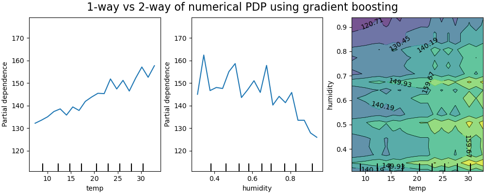
Computing partial dependence plots...
done in 8.256s

The 1D partial dependence plots for the model constrained to not model feature interactions show local spikes for each features individually, in particular for for the “humidity” feature. Those spikes might be reflecting a degraded behavior of the model that attempts to somehow compensate for the forbidden interactions by overfitting particular training points. Note that the predictive performance of this model as measured on the test set is significantly worse than that of the original, unconstrained model.

Also note that the number of local spikes visible on those plots is depends on the grid resolution parameter of the PD plot itself.

Those local spikes result in a noisily gridded 2D PD plot. It is quite challenging to tell whether or not there are no interaction between those features because of the high frequency oscillations in the humidity feature. However it can clearly be seen that the simple interaction effect observed when the temperature crosses the 20 degrees boundary is no longer visible for this model.

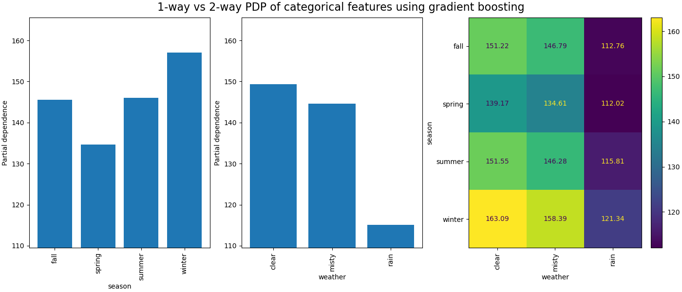
The partial dependence between categorical features will provide a discrete representation that can be shown as a heatmap. For instance the interaction between the season, the weather, and the target would be as follow:

print("Computing partial dependence plots...")
features_info = {
    "features": ["season", "weather", ("season", "weather")],
    "kind": "average",
    "categorical_features": categorical_features,
}
_, ax = plt.subplots(ncols=3, figsize=(14, 6), constrained_layout=True)
tic = time()
display = PartialDependenceDisplay.from_estimator(
    hgbdt_model,
    X_train,
    **features_info,
    ax=ax,
    **common_params,
)

print(f"done in {time() - tic:.3f}s")
_ = display.figure_.suptitle(
    "1-way vs 2-way PDP of categorical features using gradient boosting", fontsize=16
)

Computing partial dependence plots...
done in 0.751s

3D representation

Let’s make the same partial dependence plot for the 2 features interaction, this time in 3 dimensions.

# unused but required import for doing 3d projections with matplotlib < 3.2
import mpl_toolkits.mplot3d  # noqa: F401
import numpy as np

from sklearn.inspection import partial_dependence

fig = plt.figure(figsize=(5.5, 5))

features = ("temp", "humidity")
pdp = partial_dependence(
    hgbdt_model, X_train, features=features, kind="average", grid_resolution=10
)
XX, YY = np.meshgrid(pdp["grid_values"][0], pdp["grid_values"][1])
Z = pdp.average[0].T
ax = fig.add_subplot(projection="3d")
fig.add_axes(ax)

surf = ax.plot_surface(XX, YY, Z, rstride=1, cstride=1, cmap=plt.cm.BuPu, edgecolor="k")
ax.set_xlabel(features[0])
ax.set_ylabel(features[1])
fig.suptitle(
    "PD of number of bike rentals on\nthe temperature and humidity GBDT model",
    fontsize=16,
)
# pretty init view
ax.view_init(elev=22, azim=122)
clb = plt.colorbar(surf, pad=0.08, shrink=0.6, aspect=10)
clb.ax.set_title("Partial\ndependence")
plt.show()

Related examples

Advanced Plotting With Partial Dependence

Advanced Plotting With Partial Dependence

Time-related feature engineering

Time-related feature engineering

Release Highlights for scikit-learn 0.24

Release Highlights for scikit-learn 0.24

Comparing Target Encoder with Other Encoders

Comparing Target Encoder with Other Encoders