Note
Go to the end to download the full example code or to run this example in your browser via JupyterLite or Binder.
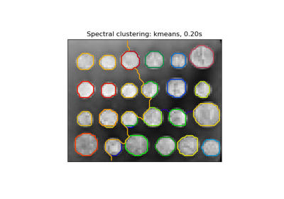
Spectral clustering for image segmentation#
In this example, an image with connected circles is generated and spectral clustering is used to separate the circles.
In these settings, the Spectral clustering approach solves the problem know as ‘normalized graph cuts’: the image is seen as a graph of connected voxels, and the spectral clustering algorithm amounts to choosing graph cuts defining regions while minimizing the ratio of the gradient along the cut, and the volume of the region.
As the algorithm tries to balance the volume (ie balance the region sizes), if we take circles with different sizes, the segmentation fails.
In addition, as there is no useful information in the intensity of the image, or its gradient, we choose to perform the spectral clustering on a graph that is only weakly informed by the gradient. This is close to performing a Voronoi partition of the graph.
In addition, we use the mask of the objects to restrict the graph to the outline of the objects. In this example, we are interested in separating the objects one from the other, and not from the background.
# Authors: The scikit-learn developers
# SPDX-License-Identifier: BSD-3-Clause
Generate the data#
import numpy as np

l = 100
x, y = np.indices((l, l))

center1 = (28, 24)
center2 = (40, 50)
center3 = (67, 58)
center4 = (24, 70)

radius1, radius2, radius3, radius4 = 16, 14, 15, 14

circle1 = (x - center1[0]) ** 2 + (y - center1[1]) ** 2 < radius1**2
circle2 = (x - center2[0]) ** 2 + (y - center2[1]) ** 2 < radius2**2
circle3 = (x - center3[0]) ** 2 + (y - center3[1]) ** 2 < radius3**2
circle4 = (x - center4[0]) ** 2 + (y - center4[1]) ** 2 < radius4**2
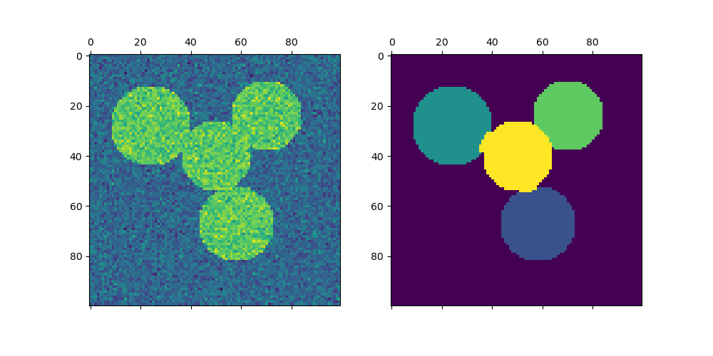
Plotting four circles#
img = circle1 + circle2 + circle3 + circle4

# We use a mask that limits to the foreground: the problem that we are
# interested in here is not separating the objects from the background,
# but separating them one from the other.
mask = img.astype(bool)

img = img.astype(float)
img += 1 + 0.2 * np.random.randn(*img.shape)
Convert the image into a graph with the value of the gradient on the edges.
from sklearn.feature_extraction import image

graph = image.img_to_graph(img, mask=mask)
Take a decreasing function of the gradient resulting in a segmentation that is close to a Voronoi partition
graph.data = np.exp(-graph.data / graph.data.std())
Here we perform spectral clustering using the arpack solver since amg is numerically unstable on this example. We then plot the results.
import matplotlib.pyplot as plt

from sklearn.cluster import spectral_clustering

labels = spectral_clustering(graph, n_clusters=4, eigen_solver="arpack")
label_im = np.full(mask.shape, -1.0)
label_im[mask] = labels

fig, axs = plt.subplots(nrows=1, ncols=2, figsize=(10, 5))
axs[0].matshow(img)
axs[1].matshow(label_im)

plt.show()
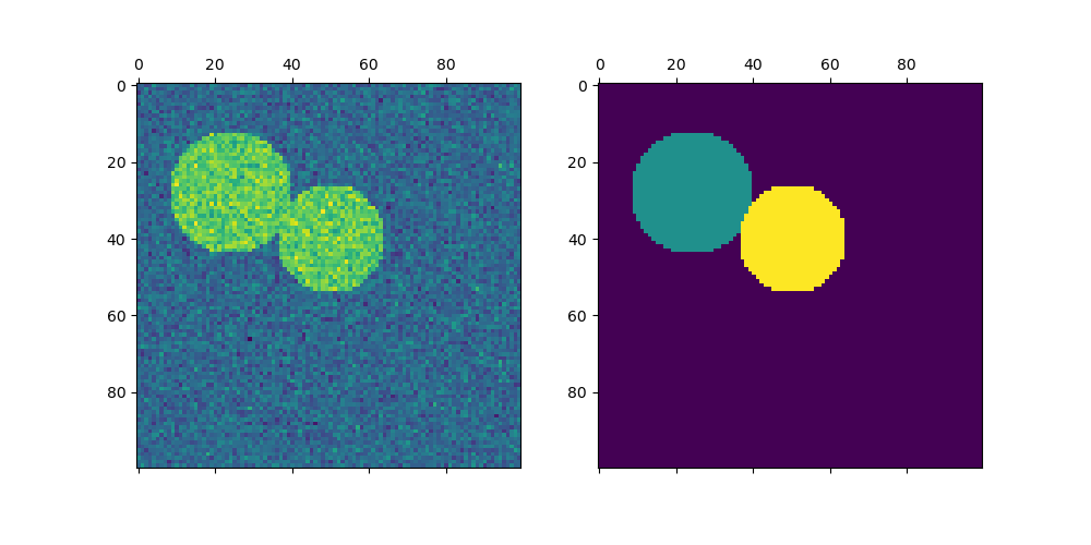
Plotting two circles#
Here we repeat the above process but only consider the first two circles we generated. Note that this results in a cleaner separation between the circles as the region sizes are easier to balance in this case.
img = circle1 + circle2
mask = img.astype(bool)
img = img.astype(float)

img += 1 + 0.2 * np.random.randn(*img.shape)

graph = image.img_to_graph(img, mask=mask)
graph.data = np.exp(-graph.data / graph.data.std())

labels = spectral_clustering(graph, n_clusters=2, eigen_solver="arpack")
label_im = np.full(mask.shape, -1.0)
label_im[mask] = labels

fig, axs = plt.subplots(nrows=1, ncols=2, figsize=(10, 5))
axs[0].matshow(img)
axs[1].matshow(label_im)

plt.show()
Total running time of the script: (0 minutes 0.222 seconds)
Related examples
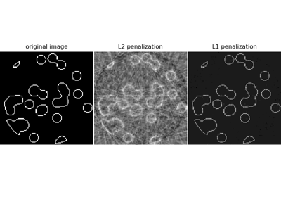
Compressive sensing: tomography reconstruction with L1 prior (Lasso)