Note
Go to the end to download the full example code or to run this example in your browser via JupyterLite or Binder.
Decision Boundaries of Multinomial and One-vs-Rest Logistic Regression#
This example compares decision boundaries of multinomial and one-vs-rest logistic regression on a 2D dataset with three classes.
We make a comparison of the decision boundaries of both methods that is equivalent
to call the method predict. In addition, we plot the hyperplanes that correspond to
the line when the probability estimate for a class is of 0.5.
# Authors: The scikit-learn developers
# SPDX-License-Identifier: BSD-3-Clause
Dataset Generation#
We generate a synthetic dataset using the make_blobs
function. The dataset consists of 1,000 samples from three different classes,
centered around [-5, 0], [0, 1.5], and [5, -1]. After generation, we apply a linear
transformation to introduce some correlation between the features to make the problem
more challenging. This results in a 2D dataset with three overlapping classes,
suitable for demonstrating the differences between multinomial and one-vs-rest
logistic regression.
import matplotlib.pyplot as plt
import numpy as np

from sklearn.datasets import make_blobs

cmap = "coolwarm"

centers = [[-5, 0], [0, 1.5], [5, -1]]
X, y = make_blobs(n_samples=1_000, centers=centers, random_state=40)
transformation = [[0.4, 0.2], [-0.4, 1.2]]
X = np.dot(X, transformation)

fig, ax = plt.subplots(figsize=(6, 4))

scatter = ax.scatter(X[:, 0], X[:, 1], c=y, cmap=cmap, edgecolor="black")
ax.set(title="Synthetic Dataset", xlabel="Feature 1", ylabel="Feature 2")
_ = ax.legend(*scatter.legend_elements(), title="Classes")
Classifier Training#
We train two different logistic regression classifiers: multinomial and one-vs-rest. The multinomial classifier handles all classes simultaneously, while the one-vs-rest approach trains a binary classifier for each class against all others.
from sklearn.linear_model import LogisticRegression
from sklearn.multiclass import OneVsRestClassifier

logistic_regression_multinomial = LogisticRegression().fit(X, y)
logistic_regression_ovr = OneVsRestClassifier(LogisticRegression()).fit(X, y)

accuracy_multinomial = logistic_regression_multinomial.score(X, y)
accuracy_ovr = logistic_regression_ovr.score(X, y)
Decision Boundaries Visualization#
Let’s visualize the decision boundaries of both models that is provided by the
method predict of the classifiers.
from sklearn.inspection import DecisionBoundaryDisplay

fig, (ax1, ax2) = plt.subplots(1, 2, figsize=(12, 5), sharex=True, sharey=True)

for model, title, ax in [
    (
        logistic_regression_multinomial,
        f"Multinomial Logistic Regression\n(Accuracy: {accuracy_multinomial:.3f})",
        ax1,
    ),
    (
        logistic_regression_ovr,
        f"One-vs-Rest Logistic Regression\n(Accuracy: {accuracy_ovr:.3f})",
        ax2,
    ),
]:
    DecisionBoundaryDisplay.from_estimator(
        model,
        X,
        ax=ax,
        response_method="predict",
        alpha=0.8,
        multiclass_colors=cmap,
    )
    scatter = ax.scatter(X[:, 0], X[:, 1], c=y, cmap=cmap, edgecolor="k")
    legend = ax.legend(*scatter.legend_elements(), title="Classes")
    ax.add_artist(legend)
    ax.set_title(title)
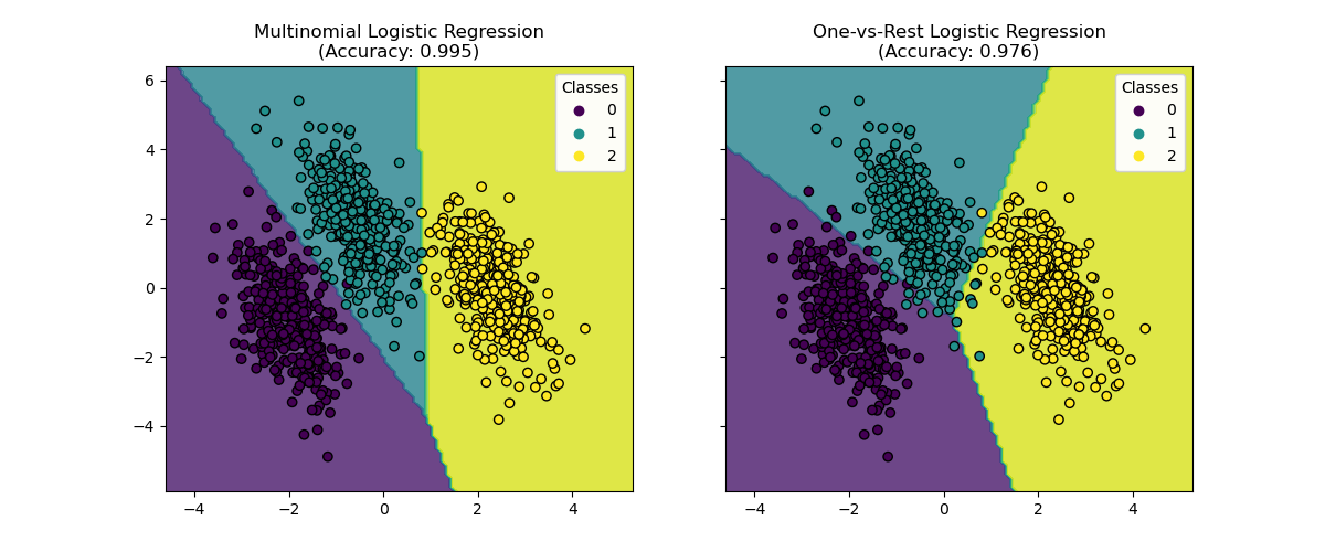
We see that the decision boundaries are different. This difference stems from their approaches:
Multinomial logistic regression considers all classes simultaneously during optimization.
One-vs-rest logistic regression fits each class independently against all others.
These distinct strategies can lead to varying decision boundaries, especially in complex multi-class problems.
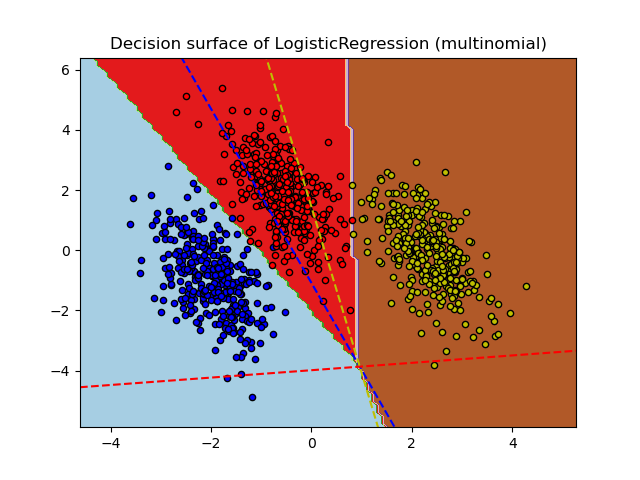
Hyperplanes Visualization#
We also visualize the hyperplanes that correspond to the line when the probability estimate for a class is 0.5.
def plot_hyperplanes(classifier, X, ax, colors):
    xmin, xmax = X[:, 0].min(), X[:, 0].max()
    ymin, ymax = X[:, 1].min(), X[:, 1].max()
    ax.set(xlim=(xmin, xmax), ylim=(ymin, ymax))

    if isinstance(classifier, OneVsRestClassifier):
        coef = np.concatenate([est.coef_ for est in classifier.estimators_])
        intercept = np.concatenate([est.intercept_ for est in classifier.estimators_])
    else:
        coef = classifier.coef_
        intercept = classifier.intercept_

    for i, color in zip(range(coef.shape[0]), colors):
        w = coef[i]
        a = -w[0] / w[1]
        xx = np.linspace(xmin, xmax)
        yy = a * xx - (intercept[i]) / w[1]
        ax.plot(xx, yy, "--", color=color, linewidth=4, label=f"Class {i}")

    return ax.get_legend_handles_labels()
fig, (ax1, ax2) = plt.subplots(1, 2, figsize=(12, 5), sharex=True, sharey=True)

for model, title, ax in [
    (
        logistic_regression_multinomial,
        "Multinomial Logistic Regression Hyperplanes",
        ax1,
    ),
    (logistic_regression_ovr, "One-vs-Rest Logistic Regression Hyperplanes", ax2),
]:
    hyperplane_handles, hyperplane_labels = plot_hyperplanes(
        model, X, ax, colors=["blue", "dimgray", "red"]
    )
    scatter = ax.scatter(X[:, 0], X[:, 1], c=y, cmap=cmap, edgecolor="k")
    scatter_handles, scatter_labels = scatter.legend_elements()

    all_handles = hyperplane_handles + scatter_handles
    all_labels = hyperplane_labels + scatter_labels

    ax.legend(all_handles, all_labels, title="Classes")
    ax.set_title(title)

plt.show()

While the hyperplanes for classes 0 and 2 are quite similar between the two methods, we observe that the hyperplane for class 1 is notably different. This difference stems from the fundamental approaches of one-vs-rest and multinomial logistic regression:
For one-vs-rest logistic regression:
Each hyperplane is determined independently by considering one class against all others.
For class 1, the hyperplane represents the decision boundary that best separates class 1 from the combined classes 0 and 2.
This binary approach can lead to simpler decision boundaries but may not capture complex relationships between all classes simultaneously.
There is no possible interpretation of the conditional class probabilities.
For multinomial logistic regression:
All hyperplanes are determined simultaneously, considering the relationships between all classes at once.
The loss minimized by the model is a proper scoring rule, which means that the model is optimized to estimate the conditional class probabilities that are, therefore, meaningful.
Each hyperplane represents the decision boundary where the probability of one class becomes higher than the others, based on the overall probability distribution.
This approach can capture more nuanced relationships between classes, potentially leading to more accurate classification in multi-class problems.
The difference in hyperplanes, especially for class 1, highlights how these methods can produce different decision boundaries despite similar overall accuracy.
In practice, using multinomial logistic regression is recommended since it minimizes a well-formulated loss function, leading to better-calibrated class probabilities and thus more interpretable results. When it comes to decision boundaries, one should formulate a utility function to transform the class probabilities into a meaningful quantity for the problem at hand. One-vs-rest allows for different decision boundaries but does not allow for fine-grained control over the trade-off between the classes as a utility function would.
Total running time of the script: (0 minutes 0.545 seconds)
Related examples
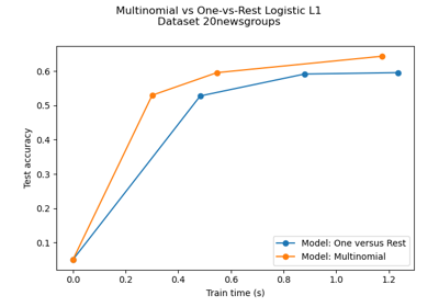
Multiclass sparse logistic regression on 20newgroups

Restricted Boltzmann Machine features for digit classification