TSNE#
- class sklearn.manifold.TSNE(n_components=2, *, perplexity=30.0, early_exaggeration=12.0, learning_rate='auto', max_iter=1000, n_iter_without_progress=300, min_grad_norm=1e-07, metric='euclidean', metric_params=None, init='pca', verbose=0, random_state=None, method='barnes_hut', angle=0.5, n_jobs=None)[source]#
T-distributed Stochastic Neighbor Embedding.
t-SNE [1] is a tool to visualize high-dimensional data. It converts similarities between data points to joint probabilities and tries to minimize the Kullback-Leibler divergence between the joint probabilities of the low-dimensional embedding and the high-dimensional data. t-SNE has a cost function that is not convex, i.e. with different initializations we can get different results.
It is highly recommended to use another dimensionality reduction method (e.g. PCA for dense data or TruncatedSVD for sparse data) to reduce the number of dimensions to a reasonable amount (e.g. 50) if the number of features is very high. This will suppress some noise and speed up the computation of pairwise distances between samples. For more tips see Laurens van der Maaten’s FAQ [2].
Read more in the User Guide.
- Parameters:
- n_componentsint, default=2
Dimension of the embedded space.
- perplexityfloat, default=30.0
The perplexity is related to the number of nearest neighbors that is used in other manifold learning algorithms. Larger datasets usually require a larger perplexity. Consider selecting a value between 5 and 50. Different values can result in significantly different results. The perplexity must be less than the number of samples.
- early_exaggerationfloat, default=12.0
Controls how tight natural clusters in the original space are in the embedded space and how much space will be between them. For larger values, the space between natural clusters will be larger in the embedded space. Again, the choice of this parameter is not very critical. If the cost function increases during initial optimization, the early exaggeration factor or the learning rate might be too high.
- learning_ratefloat or “auto”, default=”auto”
The learning rate for t-SNE is usually in the range [10.0, 1000.0]. If the learning rate is too high, the data may look like a ‘ball’ with any point approximately equidistant from its nearest neighbours. If the learning rate is too low, most points may look compressed in a dense cloud with few outliers. If the cost function gets stuck in a bad local minimum increasing the learning rate may help. Note that many other t-SNE implementations (bhtsne, FIt-SNE, openTSNE, etc.) use a definition of learning_rate that is 4 times smaller than ours. So our learning_rate=200 corresponds to learning_rate=800 in those other implementations. The ‘auto’ option sets the learning_rate to
max(N / early_exaggeration / 4, 50)where N is the sample size, following [4] and [5].Changed in version 1.2: The default value changed to
"auto".- max_iterint, default=1000
Maximum number of iterations for the optimization. Should be at least 250.
Changed in version 1.5: Parameter name changed from
n_itertomax_iter.- n_iter_without_progressint, default=300
Maximum number of iterations without progress before we abort the optimization, used after 250 initial iterations with early exaggeration. Note that progress is only checked every 50 iterations so this value is rounded to the next multiple of 50.
Added in version 0.17: parameter n_iter_without_progress to control stopping criteria.
- min_grad_normfloat, default=1e-7
If the gradient norm is below this threshold, the optimization will be stopped.
- metricstr or callable, default=’euclidean’
The metric to use when calculating distance between instances in a feature array. If metric is a string, it must be one of the options allowed by scipy.spatial.distance.pdist for its metric parameter, or a metric listed in pairwise.PAIRWISE_DISTANCE_FUNCTIONS. If metric is “precomputed”, X is assumed to be a distance matrix. Alternatively, if metric is a callable function, it is called on each pair of instances (rows) and the resulting value recorded. The callable should take two arrays from X as input and return a value indicating the distance between them. The default is “euclidean” which is interpreted as squared euclidean distance.
- metric_paramsdict, default=None
Additional keyword arguments for the metric function.
Added in version 1.1.
- init{“random”, “pca”} or ndarray of shape (n_samples, n_components), default=”pca”
Initialization of embedding. PCA initialization cannot be used with precomputed distances and is usually more globally stable than random initialization.
Changed in version 1.2: The default value changed to
"pca".- verboseint, default=0
Verbosity level.
- random_stateint, RandomState instance or None, default=None
Determines the random number generator. Pass an int for reproducible results across multiple function calls. Note that different initializations might result in different local minima of the cost function. See Glossary.
- method{‘barnes_hut’, ‘exact’}, default=’barnes_hut’
By default the gradient calculation algorithm uses Barnes-Hut approximation running in O(NlogN) time. method=’exact’ will run on the slower, but exact, algorithm in O(N^2) time. The exact algorithm should be used when nearest-neighbor errors need to be better than 3%. However, the exact method cannot scale to millions of examples.
Added in version 0.17: Approximate optimization method via the Barnes-Hut.
- anglefloat, default=0.5
Only used if method=’barnes_hut’ This is the trade-off between speed and accuracy for Barnes-Hut T-SNE. ‘angle’ is the angular size (referred to as theta in [3]) of a distant node as measured from a point. If this size is below ‘angle’ then it is used as a summary node of all points contained within it. This method is not very sensitive to changes in this parameter in the range of 0.2 - 0.8. Angle less than 0.2 has quickly increasing computation time and angle greater 0.8 has quickly increasing error.
- n_jobsint, default=None
The number of parallel jobs to run for neighbors search. This parameter has no impact when
metric="precomputed"or (metric="euclidean"andmethod="exact").Nonemeans 1 unless in ajoblib.parallel_backendcontext.-1means using all processors. See Glossary for more details.Added in version 0.22.
- Attributes:
- embedding_array-like of shape (n_samples, n_components)
Stores the embedding vectors.
- kl_divergence_float
Kullback-Leibler divergence after optimization.
- n_features_in_int
Number of features seen during fit.
Added in version 0.24.
- feature_names_in_ndarray of shape (
n_features_in_,) Names of features seen during fit. Defined only when
Xhas feature names that are all strings.Added in version 1.0.
- learning_rate_float
Effective learning rate.
Added in version 1.2.
- n_iter_int
Number of iterations run.
See also
sklearn.decomposition.PCAPrincipal component analysis that is a linear dimensionality reduction method.
sklearn.decomposition.KernelPCANon-linear dimensionality reduction using kernels and PCA.
MDSManifold learning using multidimensional scaling.
IsomapManifold learning based on Isometric Mapping.
LocallyLinearEmbeddingManifold learning using Locally Linear Embedding.
SpectralEmbeddingSpectral embedding for non-linear dimensionality.
Notes
For an example of using
TSNEin combination withKNeighborsTransformersee Approximate nearest neighbors in TSNE.References
- [1] van der Maaten, L.J.P.; Hinton, G.E. Visualizing High-Dimensional Data
Using t-SNE. Journal of Machine Learning Research 9:2579-2605, 2008.
- [2] van der Maaten, L.J.P. t-Distributed Stochastic Neighbor Embedding
- [3] L.J.P. van der Maaten. Accelerating t-SNE using Tree-Based Algorithms.
Journal of Machine Learning Research 15(Oct):3221-3245, 2014. https://lvdmaaten.github.io/publications/papers/JMLR_2014.pdf
- [4] Belkina, A. C., Ciccolella, C. O., Anno, R., Halpert, R., Spidlen, J.,
& Snyder-Cappione, J. E. (2019). Automated optimized parameters for T-distributed stochastic neighbor embedding improve visualization and analysis of large datasets. Nature Communications, 10(1), 1-12.
- [5] Kobak, D., & Berens, P. (2019). The art of using t-SNE for single-cell
transcriptomics. Nature Communications, 10(1), 1-14.
Examples
>>> import numpy as np
>>> from sklearn.manifold import TSNE
>>> X = np.array([[0, 0, 0], [0, 1, 1], [1, 0, 1], [1, 1, 1]])
>>> X_embedded = TSNE(n_components=2, learning_rate='auto',
...                   init='random', perplexity=3).fit_transform(X)
>>> X_embedded.shape
(4, 2)
- fit(X, y=None)[source]#
Fit X into an embedded space.
- Parameters:
- X{array-like, sparse matrix} of shape (n_samples, n_features) or (n_samples, n_samples)
If the metric is ‘precomputed’ X must be a square distance matrix. Otherwise it contains a sample per row. If the method is ‘exact’, X may be a sparse matrix of type ‘csr’, ‘csc’ or ‘coo’. If the method is ‘barnes_hut’ and the metric is ‘precomputed’, X may be a precomputed sparse graph.
- yNone
Ignored.
- Returns:
- selfobject
Fitted estimator.
- fit_transform(X, y=None)[source]#
Fit X into an embedded space and return that transformed output.
- Parameters:
- X{array-like, sparse matrix} of shape (n_samples, n_features) or (n_samples, n_samples)
If the metric is ‘precomputed’ X must be a square distance matrix. Otherwise it contains a sample per row. If the method is ‘exact’, X may be a sparse matrix of type ‘csr’, ‘csc’ or ‘coo’. If the method is ‘barnes_hut’ and the metric is ‘precomputed’, X may be a precomputed sparse graph.
- yNone
Ignored.
- Returns:
- X_newndarray of shape (n_samples, n_components)
Embedding of the training data in low-dimensional space.
- get_feature_names_out(input_features=None)[source]#
Get output feature names for transformation.
The feature names out will prefixed by the lowercased class name. For example, if the transformer outputs 3 features, then the feature names out are:
["class_name0", "class_name1", "class_name2"].- Parameters:
- input_featuresarray-like of str or None, default=None
Only used to validate feature names with the names seen in
fit.
- Returns:
- feature_names_outndarray of str objects
Transformed feature names.
- get_metadata_routing()[source]#
Get metadata routing of this object.
Please check User Guide on how the routing mechanism works.
- Returns:
- routingMetadataRequest
A
MetadataRequestencapsulating routing information.
- get_params(deep=True)[source]#
Get parameters for this estimator.
- Parameters:
- deepbool, default=True
If True, will return the parameters for this estimator and contained subobjects that are estimators.
- Returns:
- paramsdict
Parameter names mapped to their values.
- set_output(*, transform=None)[source]#
Set output container.
Refer to the user guide for more details and Introducing the set_output API for an example on how to use the API.
- Parameters:
- transform{“default”, “pandas”, “polars”}, default=None
Configure output of
transformandfit_transform."default": Default output format of a transformer"pandas": DataFrame output"polars": Polars outputNone: Transform configuration is unchanged
Added in version 1.4:
"polars"option was added.
- Returns:
- selfestimator instance
Estimator instance.
- set_params(**params)[source]#
Set the parameters of this estimator.
The method works on simple estimators as well as on nested objects (such as
Pipeline). The latter have parameters of the form<component>__<parameter>so that it’s possible to update each component of a nested object.- Parameters:
- **paramsdict
Estimator parameters.
- Returns:
- selfestimator instance
Estimator instance.
Gallery examples#
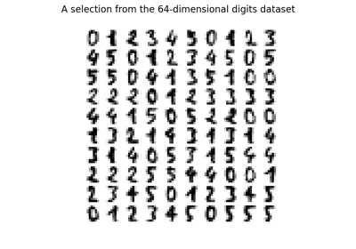
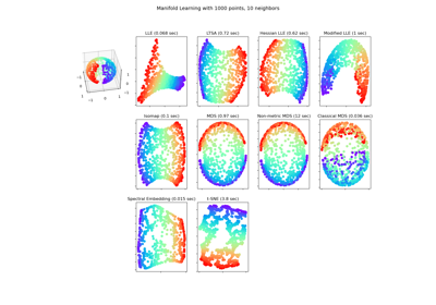
Manifold learning on handwritten digits: Locally Linear Embedding, Isomap…
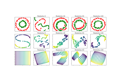
t-SNE: The effect of various perplexity values on the shape