Note

Go to the end to download the full example code or to run this example in your browser via JupyterLite or Binder.

Release Highlights for scikit-learn 1.9#

We are pleased to announce the release of scikit-learn 1.9! Many bug fixes and improvements were added, as well as some key new features. Below we detail the highlights of this release. For an exhaustive list of all the changes, please refer to the release notes.

To install the latest version (with pip):

pip install --upgrade scikit-learn

or with conda:

conda install -c conda-forge scikit-learn

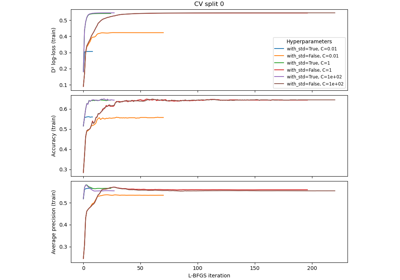
Callbacks#

This release introduces experimental support for callbacks in scikit-learn. They are objects that can be registered on estimators, through the set_callbacks method, to be invoked at the beginning and end of key steps during fit. See the user guide for more details. Only a few estimators support callbacks for now, see the list of supported estimators.

Two built-in callbacks are provided in this release:

ProgressBar, to display progress bars.
ScoringMonitor, to compute and log scoring metrics.

from sklearn.callback import ProgressBar, ScoringMonitor
from sklearn.datasets import make_classification
from sklearn.linear_model import LogisticRegression

X, y = make_classification(
    n_samples=1000, n_features=50, n_classes=10, n_informative=20, random_state=0
)

scoring_monitor = ScoringMonitor(scoring="d2_log_loss_score")
logreg = LogisticRegression(solver="lbfgs")
logreg.set_callbacks(scoring_monitor, ProgressBar())
logreg.fit(X, y)

log = scoring_monitor.get_logs().data_as_pandas
log[["task_name", "task_id", "d2_log_loss_score"]]

LogisticRegression - fit ━━━━━━━━━━━━━━━━━━━━━━━━━━━━━━━━━━━━━━━━ 100% 0:00:00

	task_name	task_id	d2_log_loss_score
0	fit	0	0.332951
1	lbfgs-iter	0	0.022579
2	lbfgs-iter	1	0.176312
3	lbfgs-iter	2	0.242118
4	lbfgs-iter	3	0.266016
...	...	...	...
60	lbfgs-iter	59	0.332950
61	lbfgs-iter	60	0.332950
62	lbfgs-iter	61	0.332950
63	lbfgs-iter	62	0.332951
64	lbfgs-iter	63	0.332951

65 rows × 3 columns

Progress bars can also be displayed for compositions of estimators.

from sklearn.callback import ProgressBar
from sklearn.datasets import load_iris
from sklearn.linear_model import LogisticRegression
from sklearn.model_selection import GridSearchCV

X, y = load_iris(return_X_y=True)
logreg = LogisticRegression(solver="lbfgs")
grid_search = GridSearchCV(logreg, {"C": [10, 1, 0.1]}, n_jobs=2)
grid_search.set_callbacks(ProgressBar())
grid_search.fit(X, y)

Intermediate output. Note that two sub-tasks progress concurrently because we set n_jobs=2:

GridSearchCV - fit                                                          ━━━━━━╸                                   17% 0:00:02
  GridSearchCV - search #0                                                  ━━━━━━━━━━━━━╸                            34% 0:00:01
    GridSearchCV - candidate-split-evaluation | LogisticRegression - fit #1 ━━━━━━━━━━━━━━━━━━━━━━━━━━━━━━━━━━━━━━━━ 100% 0:00:00
    GridSearchCV - candidate-split-evaluation | LogisticRegression - fit #0 ━━━━━━━━━━━━━━━━━━━━━━━━━━━━━━━━━━━━━━━━ 100% 0:00:00
    GridSearchCV - candidate-split-evaluation | LogisticRegression - fit #2 ━━━━━━━━━━━━━━━━━━━━━━━━━━━━━━━━━━━━━━━━ 100% 0:00:00
    GridSearchCV - candidate-split-evaluation | LogisticRegression - fit #3 ━━━━━━━━━━━━━━━━━━━━━━━━━━━━━━━━━━━━━━━━ 100% 0:00:00
    GridSearchCV - candidate-split-evaluation | LogisticRegression - fit #4 ━━━━━━━━━━━━━━━━━━━━━╸                    54% 0:00:01
    GridSearchCV - candidate-split-evaluation | LogisticRegression - fit #5 ━━━━━━━━━━━━━━━━━                         44% 0:00:01

Final output displaying all the completed nested subtasks:

GridSearchCV - fit                                                           ━━━━━━━━━━━━━━━━━━━━━━━━━━━━━━━━━━━━━━━━ 100% 0:00:00
  GridSearchCV - search #0                                                   ━━━━━━━━━━━━━━━━━━━━━━━━━━━━━━━━━━━━━━━━ 100% 0:00:00
    GridSearchCV - candidate-split-evaluation | LogisticRegression - fit #1  ━━━━━━━━━━━━━━━━━━━━━━━━━━━━━━━━━━━━━━━━ 100% 0:00:00
    GridSearchCV - candidate-split-evaluation | LogisticRegression - fit #0  ━━━━━━━━━━━━━━━━━━━━━━━━━━━━━━━━━━━━━━━━ 100% 0:00:00
    GridSearchCV - candidate-split-evaluation | LogisticRegression - fit #2  ━━━━━━━━━━━━━━━━━━━━━━━━━━━━━━━━━━━━━━━━ 100% 0:00:00
    GridSearchCV - candidate-split-evaluation | LogisticRegression - fit #3  ━━━━━━━━━━━━━━━━━━━━━━━━━━━━━━━━━━━━━━━━ 100% 0:00:00
    GridSearchCV - candidate-split-evaluation | LogisticRegression - fit #4  ━━━━━━━━━━━━━━━━━━━━━━━━━━━━━━━━━━━━━━━━ 100% 0:00:00
    GridSearchCV - candidate-split-evaluation | LogisticRegression - fit #5  ━━━━━━━━━━━━━━━━━━━━━━━━━━━━━━━━━━━━━━━━ 100% 0:00:00
    GridSearchCV - candidate-split-evaluation | LogisticRegression - fit #6  ━━━━━━━━━━━━━━━━━━━━━━━━━━━━━━━━━━━━━━━━ 100% 0:00:00
    GridSearchCV - candidate-split-evaluation | LogisticRegression - fit #7  ━━━━━━━━━━━━━━━━━━━━━━━━━━━━━━━━━━━━━━━━ 100% 0:00:00
    GridSearchCV - candidate-split-evaluation | LogisticRegression - fit #8  ━━━━━━━━━━━━━━━━━━━━━━━━━━━━━━━━━━━━━━━━ 100% 0:00:00
    GridSearchCV - candidate-split-evaluation | LogisticRegression - fit #9  ━━━━━━━━━━━━━━━━━━━━━━━━━━━━━━━━━━━━━━━━ 100% 0:00:00
    GridSearchCV - candidate-split-evaluation | LogisticRegression - fit #10 ━━━━━━━━━━━━━━━━━━━━━━━━━━━━━━━━━━━━━━━━ 100% 0:00:00
    GridSearchCV - candidate-split-evaluation | LogisticRegression - fit #11 ━━━━━━━━━━━━━━━━━━━━━━━━━━━━━━━━━━━━━━━━ 100% 0:00:00
    GridSearchCV - candidate-split-evaluation | LogisticRegression - fit #12 ━━━━━━━━━━━━━━━━━━━━━━━━━━━━━━━━━━━━━━━━ 100% 0:00:00
    GridSearchCV - candidate-split-evaluation | LogisticRegression - fit #13 ━━━━━━━━━━━━━━━━━━━━━━━━━━━━━━━━━━━━━━━━ 100% 0:00:00
    GridSearchCV - candidate-split-evaluation | LogisticRegression - fit #14 ━━━━━━━━━━━━━━━━━━━━━━━━━━━━━━━━━━━━━━━━ 100% 0:00:00
  GridSearchCV - refit-with-best-params | LogisticRegression - fit #1        ━━━━━━━━━━━━━━━━━━━━━━━━━━━━━━━━━━━━━━━━ 100% 0:00:00

There is also a public API to implement callback support in third-party estimators and to implement custom callbacks. See the developer’s guide for more details.

New callbacks and callback support in more estimators will be added in future releases. The callback API is experimental and may evolve without deprecation.

Improvements to the HTML representation of estimators#

The HTML representation of estimators now includes information made available after fit. There is a new “Fitted attributes” table that lists the fitted attributes and their type and values. In addition, the HTML representation of transformers includes new visual blocks showing the number and names of the output features.

Expand the diagram below by clicking on the different visual blocks to see the new features.

import pandas as pd

from sklearn.compose import make_column_transformer
from sklearn.linear_model import LogisticRegression
from sklearn.pipeline import make_pipeline
from sklearn.preprocessing import OneHotEncoder, StandardScaler

X = pd.DataFrame({"num": [0.1, 0.2, 0.3, 0.4], "cat": ["A", "C", "B", "C"]})
y = [1, 3, 1, 2]

pipe = make_pipeline(
    make_column_transformer((StandardScaler(), ["num"]), (OneHotEncoder(), ["cat"])),
    LogisticRegression(),
)
pipe.fit(X, y)

Pipeline(steps=[('columntransformer',
                 ColumnTransformer(transformers=[('standardscaler',
                                                  StandardScaler(), ['num']),
                                                 ('onehotencoder',
                                                  OneHotEncoder(), ['cat'])])),
                ('logisticregression', LogisticRegression())])

In a Jupyter environment, please rerun this cell to show the HTML representation or trust the notebook.
On GitHub, the HTML representation is unable to render, please try loading this page with nbviewer.org.

Pipeline

?Documentation for PipelineiFitted

Parameters

	steps steps: list of tuples List of (name of step, estimator) tuples that are to be chained in sequential order. To be compatible with the scikit-learn API, all steps must define `fit`. All non-last steps must also define `transform`. See :ref:`Combining Estimators <combining_estimators>` for more details.	[('columntransformer', ...), ('logisticregression', ...)]
	transform_input transform_input: list of str, default=None The names of the :term:`metadata` parameters that should be transformed by the pipeline before passing it to the step consuming it. This enables transforming some input arguments to ``fit`` (other than ``X``) to be transformed by the steps of the pipeline up to the step which requires them. Requirement is defined via :ref:`metadata routing <metadata_routing>`. For instance, this can be used to pass a validation set through the pipeline. You can only set this if metadata routing is enabled, which you can enable using ``sklearn.set_config(enable_metadata_routing=True)``. .. versionadded:: 1.6	None
	memory memory: str or object with the joblib.Memory interface, default=None Used to cache the fitted transformers of the pipeline. The last step will never be cached, even if it is a transformer. By default, no caching is performed. If a string is given, it is the path to the caching directory. Enabling caching triggers a clone of the transformers before fitting. Therefore, the transformer instance given to the pipeline cannot be inspected directly. Use the attribute ``named_steps`` or ``steps`` to inspect estimators within the pipeline. Caching the transformers is advantageous when fitting is time consuming. See :ref:`sphx_glr_auto_examples_neighbors_plot_caching_nearest_neighbors.py` for an example on how to enable caching.	None
	verbose verbose: bool, default=False If True, the time elapsed while fitting each step will be printed as it is completed.	False

Fitted attributes

Name	Type	Value
classes_ classes_: ndarray of shape (n_classes,) The classes labels. Only exist if the last step of the pipeline is a classifier.	ndarray[int64](3,)	[1,2,3]
feature_names_in_ feature_names_in_: ndarray of shape (`n_features_in_`,) Names of features seen during :term:`fit`. Only defined if the underlying estimator exposes such an attribute when fit. .. versionadded:: 1.0	ndarray[object](2,)	['num','cat']
n_features_in_ n_features_in_: int Number of features seen during :term:`fit`. Only defined if the underlying first estimator in `steps` exposes such an attribute when fit. .. versionadded:: 0.24	int	2

columntransformer: ColumnTransformer

?Documentation for columntransformer: ColumnTransformer

Parameters

	transformers transformers: list of tuples List of (name, transformer, columns) tuples specifying the transformer objects to be applied to subsets of the data. name : str Like in Pipeline and FeatureUnion, this allows the transformer and its parameters to be set using ``set_params`` and searched in grid search. transformer : {'drop', 'passthrough'} or estimator Estimator must support :term:`fit` and :term:`transform`. Special-cased strings 'drop' and 'passthrough' are accepted as well, to indicate to drop the columns or to pass them through untransformed, respectively. columns : str, array-like of str, int, array-like of int, array-like of bool, slice or callable Indexes the data on its second axis. Integers are interpreted as positional columns, while strings can reference DataFrame columns by name. A scalar string or int should be used where ``transformer`` expects X to be a 1d array-like (vector), otherwise a 2d array will be passed to the transformer. A callable is passed the input data `X` and can return any of the above. To select multiple columns by name or dtype, you can use :obj:`make_column_selector`.	[('standardscaler', ...), ('onehotencoder', ...)]
	remainder remainder: {'drop', 'passthrough'} or estimator, default='drop' By default, only the specified columns in `transformers` are transformed and combined in the output, and the non-specified columns are dropped. (default of ``'drop'``). By specifying ``remainder='passthrough'``, all remaining columns that were not specified in `transformers`, but present in the data passed to `fit` will be automatically passed through. This subset of columns is concatenated with the output of the transformers. For dataframes, extra columns not seen during `fit` will be excluded from the output of `transform`. By setting ``remainder`` to be an estimator, the remaining non-specified columns will use the ``remainder`` estimator. The estimator must support :term:`fit` and :term:`transform`. Note that using this feature requires that the DataFrame columns input at :term:`fit` and :term:`transform` have identical order.	'drop'
	sparse_threshold sparse_threshold: float, default=0.3 If the output of the different transformers contains sparse matrices, these will be stacked as a sparse matrix if the overall density is lower than this value. Use ``sparse_threshold=0`` to always return dense. When the transformed output consists of all dense data, the stacked result will be dense, and this keyword will be ignored.	0.3
	n_jobs n_jobs: int, default=None Number of jobs to run in parallel. ``None`` means 1 unless in a :obj:`joblib.parallel_backend` context. ``-1`` means using all processors. See :term:`Glossary <n_jobs>` for more details.	None
	transformer_weights transformer_weights: dict, default=None Multiplicative weights for features per transformer. The output of the transformer is multiplied by these weights. Keys are transformer names, values the weights.	None
	verbose verbose: bool, default=False If True, the time elapsed while fitting each transformer will be printed as it is completed.	False
	verbose_feature_names_out verbose_feature_names_out: bool, str or Callable[[str, str], str], default=True - If True, :meth:`ColumnTransformer.get_feature_names_out` will prefix all feature names with the name of the transformer that generated that feature. It is equivalent to setting `verbose_feature_names_out="{transformer_name}__{feature_name}"`. - If False, :meth:`ColumnTransformer.get_feature_names_out` will not prefix any feature names and will error if feature names are not unique. - If ``Callable[[str, str], str]``, :meth:`ColumnTransformer.get_feature_names_out` will rename all the features using the name of the transformer. The first argument of the callable is the transformer name and the second argument is the feature name. The returned string will be the new feature name. - If ``str``, it must be a string ready for formatting. The given string will be formatted using two field names: ``transformer_name`` and ``feature_name``. e.g. ``"{feature_name}__{transformer_name}"``. See :meth:`str.format` method from the standard library for more info. .. versionadded:: 1.0 .. versionchanged:: 1.6 `verbose_feature_names_out` can be a callable or a string to be formatted.	True

Fitted attributes

Name	Type	Value
feature_names_in_ feature_names_in_: ndarray of shape (`n_features_in_`,) Names of features seen during :term:`fit`. Defined only when `X` has feature names that are all strings. .. versionadded:: 1.0	ndarray[object](2,)	['num','cat']
n_features_in_ n_features_in_: int Number of features seen during :term:`fit`. Only defined if the underlying transformers expose such an attribute when fit. .. versionadded:: 0.24	int	2
named_transformers_ named_transformers_: :class:`~sklearn.utils.Bunch` Read-only attribute to access any transformer by given name. Keys are transformer names and values are the fitted transformer objects.	Bunch	{'standardsca...eHotEncoder()}
output_indices_ output_indices_: dict A dictionary from each transformer name to a slice, where the slice corresponds to indices in the transformed output. This is useful to inspect which transformer is responsible for which transformed feature(s). .. versionadded:: 1.0	dict	{'on...er': slice(1, 4, None), 're...er': slice(0, 0, None), 'st...er': slice(0, 1, None)}
sparse_output_ sparse_output_: bool Boolean flag indicating whether the output of ``transform`` is a sparse matrix or a dense numpy array, which depends on the output of the individual transformers and the `sparse_threshold` keyword.	bool	False
transformers_ transformers_: list The collection of fitted transformers as tuples of (name, fitted_transformer, column). `fitted_transformer` can be an estimator, or `'drop'`; `'passthrough'` is replaced with an equivalent :class:`~sklearn.preprocessing.FunctionTransformer`. In case there were no columns selected, this will be the unfitted transformer. If there are remaining columns, the final element is a tuple of the form: ('remainder', transformer, remaining_columns) corresponding to the ``remainder`` parameter. If there are remaining columns, then ``len(transformers_)==len(transformers)+1``, otherwise ``len(transformers_)==len(transformers)``. .. versionadded:: 1.7 The format of the remaining columns now attempts to match that of the other transformers: if all columns were provided as column names (`str`), the remaining columns are stored as column names; if all columns were provided as mask arrays (`bool`), so are the remaining columns; in all other cases the remaining columns are stored as indices (`int`).	list	[('st...er', StandardScaler(), ['num']), ('on...er', OneHotEncoder(), ['cat'])]

standardscaler

['num']

StandardScaler

?Documentation for StandardScaler

Parameters

	copy copy: bool, default=True If False, try to avoid a copy and do inplace scaling instead. This is not guaranteed to always work inplace; e.g. if the data is not a NumPy array or scipy.sparse CSR matrix, a copy may still be returned.	True
	with_mean with_mean: bool, default=True If True, center the data before scaling. This does not work (and will raise an exception) when attempted on sparse matrices, because centering them entails building a dense matrix which in common use cases is likely to be too large to fit in memory.	True
	with_std with_std: bool, default=True If True, scale the data to unit variance (or equivalently, unit standard deviation).	True

Fitted attributes

Name	Type	Value
feature_names_in_ feature_names_in_: ndarray of shape (`n_features_in_`,) Names of features seen during :term:`fit`. Defined only when `X` has feature names that are all strings. .. versionadded:: 1.0	ndarray[object](1,)	['num']
mean_ mean_: ndarray of shape (n_features,) or None The mean value for each feature in the training set. Equal to ``None`` when ``with_mean=False`` and ``with_std=False``.	ndarray[float64](1,)	[0.25]
n_features_in_ n_features_in_: int Number of features seen during :term:`fit`. .. versionadded:: 0.24	int	1
n_samples_seen_ n_samples_seen_: int or ndarray of shape (n_features,) The number of samples processed by the estimator for each feature. If there are no missing samples, the ``n_samples_seen`` will be an integer, otherwise it will be an array of dtype int. If `sample_weights` are used it will be a float (if no missing data) or an array of dtype float that sums the weights seen so far. Will be reset on new calls to fit, but increments across ``partial_fit`` calls.	float64	4
scale_ scale_: ndarray of shape (n_features,) or None Per feature relative scaling of the data to achieve zero mean and unit variance. Generally this is calculated using `np.sqrt(var_)`. If a variance is zero, we can't achieve unit variance, and the data is left as-is, giving a scaling factor of 1. `scale_` is equal to `None` when `with_std=False`. .. versionadded:: 0.17 scale_	ndarray[float64](1,)	[0.11]
var_ var_: ndarray of shape (n_features,) or None The variance for each feature in the training set. Used to compute `scale_`. Equal to ``None`` when ``with_mean=False`` and ``with_std=False``.	ndarray[float64](1,)	[0.01]

1 feature

num

onehotencoder

['cat']

OneHotEncoder

?Documentation for OneHotEncoder

Parameters

	categories categories: 'auto' or a list of array-like, default='auto' Categories (unique values) per feature: - 'auto' : Determine categories automatically from the training data. - list : ``categories[i]`` holds the categories expected in the ith column. The passed categories should not mix strings and numeric values within a single feature, and should be sorted in case of numeric values. The used categories can be found in the ``categories_`` attribute. .. versionadded:: 0.20	'auto'
	drop drop: {'first', 'if_binary'} or an array-like of shape (n_features,), default=None Specifies a methodology to use to drop one of the categories per feature. This is useful in situations where perfectly collinear features cause problems, such as when feeding the resulting data into an unregularized linear regression model. However, dropping one category breaks the symmetry of the original representation and can therefore induce a bias in downstream models, for instance for penalized linear classification or regression models. - None : retain all features (the default). - 'first' : drop the first category in each feature. If only one category is present, the feature will be dropped entirely. - 'if_binary' : drop the first category in each feature with two categories. Features with 1 or more than 2 categories are left intact. - array : ``drop[i]`` is the category in feature ``X[:, i]`` that should be dropped. When `max_categories` or `min_frequency` is configured to group infrequent categories, the dropping behavior is handled after the grouping. .. versionadded:: 0.21 The parameter `drop` was added in 0.21. .. versionchanged:: 0.23 The option `drop='if_binary'` was added in 0.23. .. versionchanged:: 1.1 Support for dropping infrequent categories.	None
	sparse_output sparse_output: bool, default=True When ``True``, it returns a SciPy sparse matrix/array in "Compressed Sparse Row" (CSR) format. .. versionadded:: 1.2 `sparse` was renamed to `sparse_output`	True
	dtype dtype: number type, default=np.float64 Desired dtype of output.	<class 'numpy.float64'>
	handle_unknown handle_unknown: {'error', 'ignore', 'infrequent_if_exist', 'warn'}, default='error' Specifies the way unknown categories are handled during :meth:`transform`. - 'error' : Raise an error if an unknown category is present during transform. - 'ignore' : When an unknown category is encountered during transform, the resulting one-hot encoded columns for this feature will be all zeros. In the inverse transform, an unknown category will be denoted as None. - 'infrequent_if_exist' : When an unknown category is encountered during transform, the resulting one-hot encoded columns for this feature will map to the infrequent category if it exists. The infrequent category will be mapped to the last position in the encoding. During inverse transform, an unknown category will be mapped to the category denoted `'infrequent'` if it exists. If the `'infrequent'` category does not exist, then :meth:`transform` and :meth:`inverse_transform` will handle an unknown category as with `handle_unknown='ignore'`. Infrequent categories exist based on `min_frequency` and `max_categories`. Read more in the :ref:`User Guide <encoder_infrequent_categories>`. - 'warn' : When an unknown category is encountered during transform a warning is issued, and the encoding then proceeds as described for `handle_unknown="infrequent_if_exist"`. .. versionchanged:: 1.1 `'infrequent_if_exist'` was added to automatically handle unknown categories and infrequent categories. .. versionadded:: 1.6 The option `"warn"` was added in 1.6.	'error'
	min_frequency min_frequency: int or float, default=None Specifies the minimum frequency below which a category will be considered infrequent. - If `int`, categories with a smaller cardinality will be considered infrequent. - If `float`, categories with a smaller cardinality than `min_frequency * n_samples` will be considered infrequent. .. versionadded:: 1.1 Read more in the :ref:`User Guide <encoder_infrequent_categories>`.	None
	max_categories max_categories: int, default=None Specifies an upper limit to the number of output features for each input feature when considering infrequent categories. If there are infrequent categories, `max_categories` includes the category representing the infrequent categories along with the frequent categories. If `None`, there is no limit to the number of output features. .. versionadded:: 1.1 Read more in the :ref:`User Guide <encoder_infrequent_categories>`.	None
	feature_name_combiner feature_name_combiner: "concat" or callable, default="concat" Callable with signature `def callable(input_feature, category)` that returns a string. This is used to create feature names to be returned by :meth:`get_feature_names_out`. `"concat"` concatenates encoded feature name and category with `feature + "_" + str(category)`.E.g. feature X with values 1, 6, 7 create feature names `X_1, X_6, X_7`. .. versionadded:: 1.3	'concat'

Fitted attributes

Name	Type	Value
categories_ categories_: list of arrays The categories of each feature determined during fitting (in order of the features in X and corresponding with the output of ``transform``). This includes the category specified in ``drop`` (if any).	list	[array(['A', '... dtype=object)]
drop_idx_ drop_idx_: array of shape (n_features,) - ``drop_idx_[i]`` is the index in ``categories_[i]`` of the category to be dropped for each feature. - ``drop_idx_[i] = None`` if no category is to be dropped from the feature with index ``i``, e.g. when `drop='if_binary'` and the feature isn't binary. - ``drop_idx_ = None`` if all the transformed features will be retained. If infrequent categories are enabled by setting `min_frequency` or `max_categories` to a non-default value and `drop_idx[i]` corresponds to an infrequent category, then the entire infrequent category is dropped. .. versionchanged:: 0.23 Added the possibility to contain `None` values.	NoneType	None
feature_names_in_ feature_names_in_: ndarray of shape (`n_features_in_`,) Names of features seen during :term:`fit`. Defined only when `X` has feature names that are all strings. .. versionadded:: 1.0	ndarray[object](1,)	['cat']
n_features_in_ n_features_in_: int Number of features seen during :term:`fit`. .. versionadded:: 1.0	int	1

3 features

cat_A

cat_B

cat_C

4 features

standardscaler__num

onehotencoder__cat_A

onehotencoder__cat_B

onehotencoder__cat_C

LogisticRegression

?Documentation for LogisticRegression

Parameters

	penalty penalty: {'l1', 'l2', 'elasticnet', None}, default='l2' Specify the norm of the penalty: - `None`: no penalty is added; - `'l2'`: add an L2 penalty term and it is the default choice; - `'l1'`: add an L1 penalty term; - `'elasticnet'`: both L1 and L2 penalty terms are added. .. warning:: Some penalties may not work with some solvers. See the parameter `solver` below, to know the compatibility between the penalty and solver. .. versionadded:: 0.19 l1 penalty with SAGA solver (allowing 'multinomial' + L1) .. deprecated:: 1.8 `penalty` was deprecated in version 1.8 and will be removed in 1.10. Use `l1_ratio` and `C` instead. `l1_ratio=0` for `penalty='l2'`, `l1_ratio=1` for `penalty='l1'`, `l1_ratio` set to any float between 0 and 1 for `penalty='elasticnet'`, and `C=np.inf` for `penalty=None`.	'deprecated'
	C C: float, default=1.0 Inverse of regularization strength; must be a positive float. Like in support vector machines, smaller values specify stronger regularization. `C=np.inf` results in unpenalized logistic regression. For a visual example on the effect of tuning the `C` parameter with an L1 penalty, see: :ref:`sphx_glr_auto_examples_linear_model_plot_logistic_path.py`.	1.0
	l1_ratio l1_ratio: float, default=0.0 The Elastic-Net mixing parameter, with `0 <= l1_ratio <= 1`. Setting `l1_ratio=1` gives a pure L1-penalty, setting `l1_ratio=0` a pure L2-penalty. Any value between 0 and 1 gives an Elastic-Net penalty of the form `l1_ratio * L1 + (1 - l1_ratio) * L2`. .. warning:: Certain values of `l1_ratio`, i.e. some penalties, may not work with some solvers. See the parameter `solver` below, to know the compatibility between the penalty and solver. .. versionchanged:: 1.8 Default value changed from None to 0.0. .. deprecated:: 1.8 `None` is deprecated and will be removed in version 1.10. Always use `l1_ratio` to specify the penalty type.	0.0
	dual dual: bool, default=False Dual (constrained) or primal (regularized, see also :ref:`this equation <regularized-logistic-loss>`) formulation. Dual formulation is only implemented for l2 penalty with liblinear solver. Prefer `dual=False` when n_samples > n_features.	False
	tol tol: float, default=1e-4 Tolerance for stopping criteria.	0.0001
	fit_intercept fit_intercept: bool, default=True Specifies if a constant (a.k.a. bias or intercept) should be added to the decision function.	True
	intercept_scaling intercept_scaling: float, default=1 Useful only when the solver `liblinear` is used and `self.fit_intercept` is set to `True`. In this case, `x` becomes `[x, self.intercept_scaling]`, i.e. a "synthetic" feature with constant value equal to `intercept_scaling` is appended to the instance vector. The intercept becomes ``intercept_scaling * synthetic_feature_weight``. .. note:: The synthetic feature weight is subject to L1 or L2 regularization as all other features. To lessen the effect of regularization on synthetic feature weight (and therefore on the intercept) `intercept_scaling` has to be increased.	1
	class_weight class_weight: dict or 'balanced', default=None Weights associated with classes in the form ``{class_label: weight}``. If not given, all classes are supposed to have weight one. The "balanced" mode uses the values of y to automatically adjust weights inversely proportional to class frequencies in the input data as ``n_samples / (n_classes * np.bincount(y))``. Note that these weights will be multiplied with sample_weight (passed through the fit method) if sample_weight is specified. .. versionadded:: 0.17 class_weight='balanced'	None
	random_state random_state: int, RandomState instance, default=None Used when ``solver`` == 'sag', 'saga' or 'liblinear' to shuffle the data. See :term:`Glossary <random_state>` for details.	None
	solver solver: {'lbfgs', 'liblinear', 'newton-cg', 'newton-cholesky', 'sag', 'saga'}, default='lbfgs' Algorithm to use in the optimization problem. Default is 'lbfgs'. To choose a solver, you might want to consider the following aspects: - 'lbfgs' is a good default solver because it works reasonably well for a wide class of problems. - For :term:`multiclass` problems (`n_classes >= 3`), all solvers except 'liblinear' minimize the full multinomial loss, 'liblinear' will raise an error. - 'newton-cholesky' is a good choice for `n_samples` >> `n_features * n_classes`, especially with one-hot encoded categorical features with rare categories. Be aware that the memory usage of this solver has a quadratic dependency on `n_features * n_classes` because it explicitly computes the full Hessian matrix. - For small datasets, 'liblinear' is a good choice, whereas 'sag' and 'saga' are faster for large ones; - 'liblinear' can only handle binary classification by default. To apply a one-versus-rest scheme for the multiclass setting one can wrap it with the :class:`~sklearn.multiclass.OneVsRestClassifier`. .. warning:: The choice of the algorithm depends on the penalty chosen (`l1_ratio=0` for L2-penalty, `l1_ratio=1` for L1-penalty and `0 < l1_ratio < 1` for Elastic-Net) and on (multinomial) multiclass support: ================= ======================== ====================== solver l1_ratio multinomial multiclass ================= ======================== ====================== 'lbfgs' l1_ratio=0 yes 'liblinear' l1_ratio=1 or l1_ratio=0 no 'newton-cg' l1_ratio=0 yes 'newton-cholesky' l1_ratio=0 yes 'sag' l1_ratio=0 yes 'saga' 0<=l1_ratio<=1 yes ================= ======================== ====================== .. note:: 'sag' and 'saga' fast convergence is only guaranteed on features with approximately the same scale. You can preprocess the data with a scaler from :mod:`sklearn.preprocessing`. .. seealso:: Refer to the :ref:`User Guide <Logistic_regression>` for more information regarding :class:`LogisticRegression` and more specifically the :ref:`Table <logistic_regression_solvers>` summarizing solver/penalty supports. .. versionadded:: 0.17 Stochastic Average Gradient (SAG) descent solver. Multinomial support in version 0.18. .. versionadded:: 0.19 SAGA solver. .. versionchanged:: 0.22 The default solver changed from 'liblinear' to 'lbfgs' in 0.22. .. versionadded:: 1.2 newton-cholesky solver. Multinomial support in version 1.6.	'lbfgs'
	max_iter max_iter: int, default=100 Maximum number of iterations taken for the solvers to converge.	100
	verbose verbose: int, default=0 For the liblinear and lbfgs solvers set verbose to any positive number for verbosity.	0
	warm_start warm_start: bool, default=False When set to True, reuse the solution of the previous call to fit as initialization, otherwise, just erase the previous solution. Useless for liblinear solver. See :term:`the Glossary <warm_start>`. .. versionadded:: 0.17 warm_start to support lbfgs, newton-cg, sag, saga solvers.	False
	n_jobs n_jobs: int, default=None Does not have any effect. .. deprecated:: 1.8 `n_jobs` is deprecated in version 1.8 and will be removed in 1.10.	None

Fitted attributes

Name	Type	Value
classes_ classes_: ndarray of shape (n_classes, ) A list of class labels known to the classifier.	ndarray[int64](3,)	[1,2,3]
coef_ coef_: ndarray or CSR matrix of shape (1, n_features) or (n_classes, n_features) Coefficients of the features in the decision function. `coef_` is of shape (1, n_features) when the given problem is binary. By default, it will be created as a dense array, but can be turned to sparse (CSR format) through :meth:`sparsify` (which can be beneficial under L1 regularization when many coefficients are zero), and back to dense through :meth:`densify`.	ndarray[float64](3, 4)	[[-0.3 , 0.25, 0.35,-0.6 ], [ 0.64,-0.05,-0.19, 0.24], [-0.34,-0.2 ,-0.16, 0.36]]
intercept_ intercept_: ndarray of shape (1,) or (n_classes,) Intercept (a.k.a. bias) added to the decision function. If `fit_intercept` is set to False, the intercept is set to zero. `intercept_` is of shape (1,) when the given problem is binary.	ndarray[float64](3,)	[ 0.67,-0.45,-0.22]
n_features_in_ n_features_in_: int Number of features seen during :term:`fit`. .. versionadded:: 0.24	int	4
n_iter_ n_iter_: ndarray of shape (1, ) Actual number of iterations for all classes. .. versionchanged:: 0.20 In SciPy <= 1.0.0 the number of lbfgs iterations may exceed ``max_iter``. ``n_iter_`` will now report at most ``max_iter``.	ndarray[int32](1,)	[10]

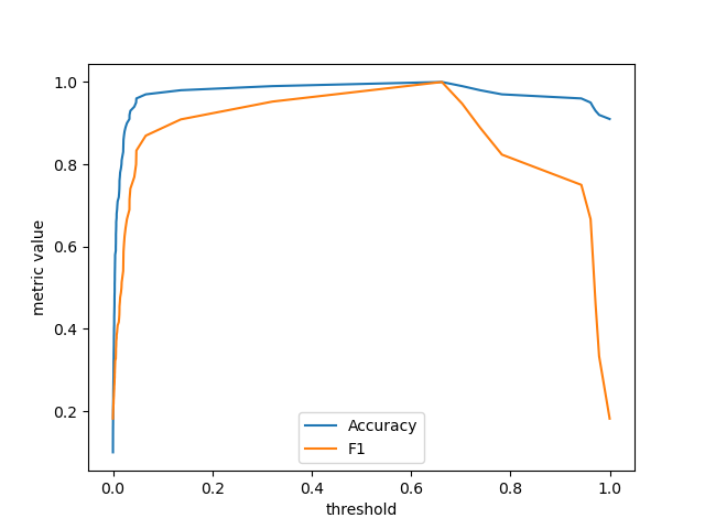
Computing metrics across thresholds#

A new function metric_at_thresholds has been added to compute an arbitrary binary classification metric across all possible decision thresholds.

import matplotlib.pyplot as plt

from sklearn.datasets import make_classification
from sklearn.linear_model import LogisticRegression
from sklearn.metrics import accuracy_score, f1_score, metric_at_thresholds

X, y = make_classification(weights=[0.9, 0.1], random_state=0)
lr = LogisticRegression(random_state=0).fit(X, y)
y_score = lr.predict_proba(X)[:, 1]

accuracy, thresholds = metric_at_thresholds(y, y_score, accuracy_score)
f1, _ = metric_at_thresholds(y, y_score, f1_score)

_, ax = plt.subplots()
ax.plot(thresholds, accuracy, label="Accuracy")
ax.plot(thresholds, f1, label="F1")
ax.set_xlabel("threshold")
ax.set_ylabel("metric value")
ax.legend()
plt.show()

Sparse array configuration#

A new configuration key "sparse_interface" has been added to control the type of sparse objects produced by functions and estimators. It is now possible to produce sparse arrays instead of sparse matrices (default). This continues the effort to prepare for SciPy’s migration from sparse matrices to sparse arrays.

import sklearn
from sklearn.preprocessing import OneHotEncoder

X = [["fox", "dog", "cat"]]
ohe = OneHotEncoder()

with sklearn.config_context(sparse_interface="sparray"):
    Xt = ohe.fit_transform(X)
Xt

<Compressed Sparse Row sparse array of dtype 'float64'
    with 3 stored elements and shape (1, 3)>

Total running time of the script: (0 minutes 0.665 seconds)

Related examples

Release Highlights for scikit-learn 1.7

Comparing randomized search and grid search for hyperparameter estimation

Release Highlights for scikit-learn 0.24

Analysis of the convergence of penalized logistic regression models

Gallery generated by Sphinx-Gallery