
Note
Go to the end to download the full example code or to run this example in your browser via JupyterLite or Binder.
Probability Calibration for 3-class classification#
This example illustrates how post-hoc calibration changes predicted probabilities for a 3-class classification problem. Illustrated is the standard 2-simplex, where the three corners correspond to the three classes. Arrows point from the probability vectors predicted by an uncalibrated classifier to the probability vectors predicted by the same classifier after calibration on a hold-out validation set. Colors indicate the true class of an instance (red: class 1, green: class 2, blue: class 3).
# Authors: The scikit-learn developers
# SPDX-License-Identifier: BSD-3-Clause
Data#
Below, we generate a classification dataset with 3 target classes so that we can visualize the probability simplex of probabilistic classifiers in a 2D plot. We then split the data into three subsets: a training set, a calibration set and a test set.
We use a large test set to get reliable estimates of the Brier score and log loss values.
To simplify the example, we use a fixed calibration set that is as large as
the training set. In practice, this would limit the amount of data available
for training the classifier and instead we would be better off using an
ensemble of calibrated classifiers using the internal cross-validation of
CalibratedClassifierCV.
Similarly, we use a large test set to get reliable estimates of the log loss and Brier score values. In practice, we would be better off using an outer cross-validation loop with the majority of the data used for training and calibration to get better models, and the rest for evaluation, at the cost of larger uncertainty in the cross-validation scores.
import numpy as np

from sklearn.datasets import make_blobs

n_train = 1_000
n_cal = 1_000
n_test = 30_000
X, y = make_blobs(
    n_samples=n_train + n_cal + n_test,
    n_features=2,
    centers=3,  # 3 classes to represent the simplex in 2D
    cluster_std=5.0,
    shuffle=True,
    random_state=42,
)
X_train, y_train = X[:n_train], y[:n_train]
X_cal, y_cal = X[n_train : n_train + n_cal], y[n_train : n_train + n_cal]
X_test, y_test = X[n_train + n_cal :], y[n_train + n_cal :]
Fitting and calibration#
First, we will train a base classifier that is expected to be poorly calibrated.
from sklearn.ensemble import RandomForestClassifier

clf = RandomForestClassifier(max_depth=7, random_state=0)
clf.fit(X_train, y_train)
Then we re-calibrate the model in a 2-stage process by fitting a sigmoid correction
to the predicted probabilities of the validation set. The sigmoid calibration is done
using the CalibratedClassifierCV. The
FrozenEstimator is used to freeze the fitted classifier to
avoid re-fitting it when calling the
fit method. This way, we
ensure that the calibration data is not used to fit the base classifier.
from sklearn.calibration import CalibratedClassifierCV
from sklearn.frozen import FrozenEstimator

cal_clf = CalibratedClassifierCV(FrozenEstimator(clf), method="sigmoid")
cal_clf.fit(X_cal, y_cal)
Compare probabilities#
Below we plot a 2-simplex with arrows showing the change in predicted probabilities on some test data points.
import matplotlib.pyplot as plt


def plot_simplex(
    p_source,
    p_target,
    color_indices,
    class_colors=["r", "g", "b"],
    arrow_alpha=0.2,
    grid_alpha=0.1,
    max_arrows=500,
    annotate=False,
    title=None,
    display_legend=True,
    ax=None,
):
    """Plot a simplex with arrows from p_source to p_target."""
    if ax is None:
        _, ax = plt.subplots(figsize=(10, 10))
    for i in range(min(p_source.shape[0], max_arrows)):
        # Normalize the source and target probabilities to ensure they are in
        # the simplex.
        p_source[i] /= p_source[i].sum()
        p_target[i] /= p_target[i].sum()

        # Plot the arrow from source to target.
        ax.arrow(
            p_source[i, 0],
            p_source[i, 1],
            p_target[i, 0] - p_source[i, 0],
            p_target[i, 1] - p_source[i, 1],
            color=class_colors[color_indices[i]],
            head_width=1e-2,
            alpha=arrow_alpha,
        )

    # Plot perfect predictions, at each vertex
    ax.plot([1.0], [0.0], "ro", ms=10, label="Class 1")
    ax.plot([0.0], [1.0], "go", ms=10, label="Class 2")
    ax.plot([0.0], [0.0], "bo", ms=10, label="Class 3")

    # Plot boundaries of unit simplex
    ax.plot([0.0, 1.0, 0.0, 0.0], [0.0, 0.0, 1.0, 0.0], "k", label="Simplex")

    # Annotate points 6 points around the simplex, and mid point inside simplex
    if annotate:
        arrow_props = dict(facecolor="black", width=2.0, headwidth=7.0)
        for text, xy, xytext in [
            (
                r"($\frac{1}{3}$, $\frac{1}{3}$, $\frac{1}{3}$)",
                (1.0 / 3, 1.0 / 3),
                (1.0 / 3, 0.23),
            ),
            (r"($\frac{1}{2}$, $0$, $\frac{1}{2}$)", (0.5, 0.0), (0.5, 0.1)),
            (r"($0$, $\frac{1}{2}$, $\frac{1}{2}$)", (0.0, 0.5), (0.1, 0.5)),
            (r"($\frac{1}{2}$, $\frac{1}{2}$, $0$)", (0.5, 0.5), (0.6, 0.6)),
            (r"($0$, $0$, $1$)", (0, 0), (0.1, 0.1)),
            (r"($1$, $0$, $0$)", (1, 0), (1, 0.1)),
            (r"($0$, $1$, $0$)", (0, 1), (0.1, 1)),
        ]:
            ax.annotate(
                text,
                xy=xy,
                xytext=xytext,
                xycoords="data",
                arrowprops=arrow_props,
                horizontalalignment="center",
                verticalalignment="center",
            )

    # Add grid
    ax.grid(False)
    for x in np.linspace(0, 1, 11):
        ax.plot([0, x], [x, 0], "k", alpha=grid_alpha)
        ax.plot([0, 0 + (1 - x) / 2], [x, x + (1 - x) / 2], "k", alpha=grid_alpha)
        ax.plot([x, x + (1 - x) / 2], [0, 0 + (1 - x) / 2], "k", alpha=grid_alpha)

    ax.set(
        title=title,
        xlabel="Probability class 1",
        ylabel="Probability class 2",
        xlim=(-0.05, 1.05),
        ylim=(-0.05, 1.05),
        aspect="equal",
    )
    if display_legend:
        ax.legend(loc="best")


uncal_clf_probs = clf.predict_proba(X_test)
cal_clf_probs = cal_clf.predict_proba(X_test)

plot_simplex(
    uncal_clf_probs,
    cal_clf_probs,
    y_test,
    annotate=True,
    title="Change of predicted probabilities on test samples after sigmoid calibration",
)
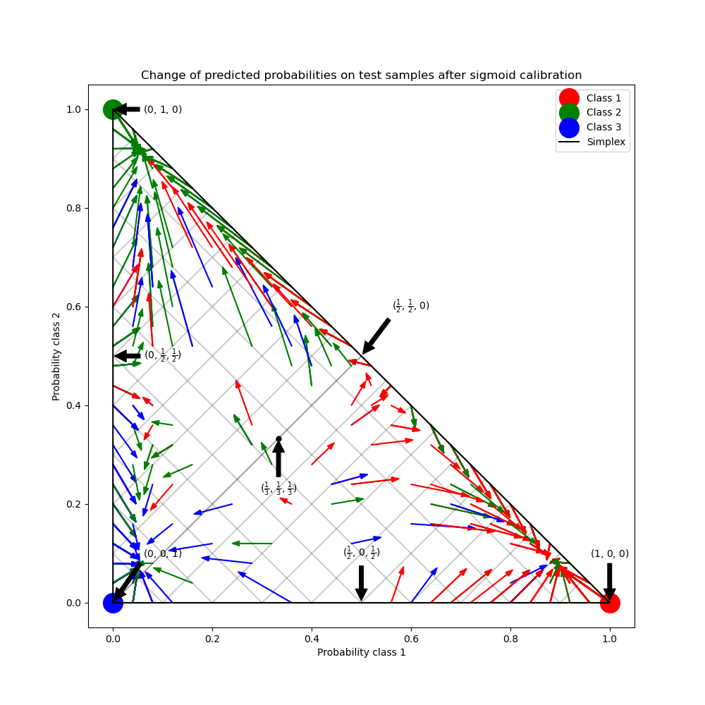
In the figure above, each vertex of the simplex represents a predicted class with maximum confidence (e.g., 1, 0, 0). The mid point inside the simplex represents predicting the three classes with equal probability (i.e., 1/3, 1/3, 1/3). Each arrow starts at the uncalibrated probabilities and end with the arrow head at the calibrated probabilities. The color of the arrow represents the true class of that test sample.
Notice in the figure above that the arrows generally point away from the edges of the simplex, where the probability of one class is 0. This results in fewer over-confident (near 0 or 1) predicted probabilities.
In this example, the re-calibration yields an overall better model. We can show
this objectively by comparing the log loss (lower is better)
of the uncalibrated and re-calibrated classifiers on the predictions of the test
set. Note that an alternative would have been to increase the number
of base estimators (trees) of the
RandomForestClassifier which could have resulted in
a similar decrease in log loss.
Log-loss of:
 - uncalibrated classifier: 0.441
 - calibrated classifier: 0.436
We can also assess model quality with the Brier score for probabilistic predictions (lower is better, possible range is [0, 2]):
from sklearn.metrics import brier_score_loss

loss = brier_score_loss(y_test, uncal_clf_probs)
cal_loss = brier_score_loss(y_test, cal_clf_probs)

print("Brier score of")
print(f" - uncalibrated classifier: {loss:.3f}")
print(f" - calibrated classifier: {cal_loss:.3f}")
Brier score of
 - uncalibrated classifier: 0.249
 - calibrated classifier: 0.248
According to the Brier score, the calibrated classifier is also slightly better than the original model.
Be aware that an improvement in log loss or Brier score on a test set is not always guaranteed.
Finally, we generate a grid of uncalibrated probabilities over the 2-simplex, compute the corresponding calibrated probabilities and plot arrows for each. The arrows are colored according the highest uncalibrated probability. This illustrates the learned calibration map:
from sklearn.calibration import _ensure_logits


def plot_calibrator_map(cal_clf, **kwargs):
    # Generate grid of probability values
    eps = np.finfo(np.float64).eps
    p1d = np.linspace(0, 1, 21)
    p0, p1 = np.meshgrid(p1d, p1d)
    p2 = 1 - p0 - p1
    original_probability = np.c_[p0.ravel(), p1.ravel(), p2.ravel()]
    original_probability = original_probability[original_probability[:, 2] >= 0]
    original_probability = original_probability.clip(eps, 1 - eps)

    method = cal_clf.method
    calibrators = cal_clf.calibrated_classifiers_[0].calibrators
    logits = _ensure_logits(
        original_probability, response_method_name="predict_proba", method=method
    )

    if method in ("sigmoid", "isotonic"):
        # Use the class-wise OvR calibrators to compute calibrated probabilities.
        calibrated_predictions = np.vstack(
            [
                calibrator.predict(logit_for_class)
                for calibrator, logit_for_class in zip(calibrators, logits.T)
            ]
        ).T
        # Re-normalize the calibrated predictions to make sure they stay inside the
        # simplex. This same renormalization step is performed internally by the
        # predict method of CalibratedClassifierCV on multiclass problems.
        calibrated_predictions /= calibrated_predictions.sum(axis=1)[:, None]
    elif method == "temperature":
        calibrated_predictions = calibrators[0].predict(logits)
    else:
        raise ValueError(
            f"Unknown calibration method: {method}. "
            "Expected 'sigmoid', 'isotonic', or 'temperature'."
        )

    plot_simplex(
        original_probability,
        calibrated_predictions,
        np.argmax(original_probability, axis=1),
        **kwargs,
    )


plot_calibrator_map(cal_clf)
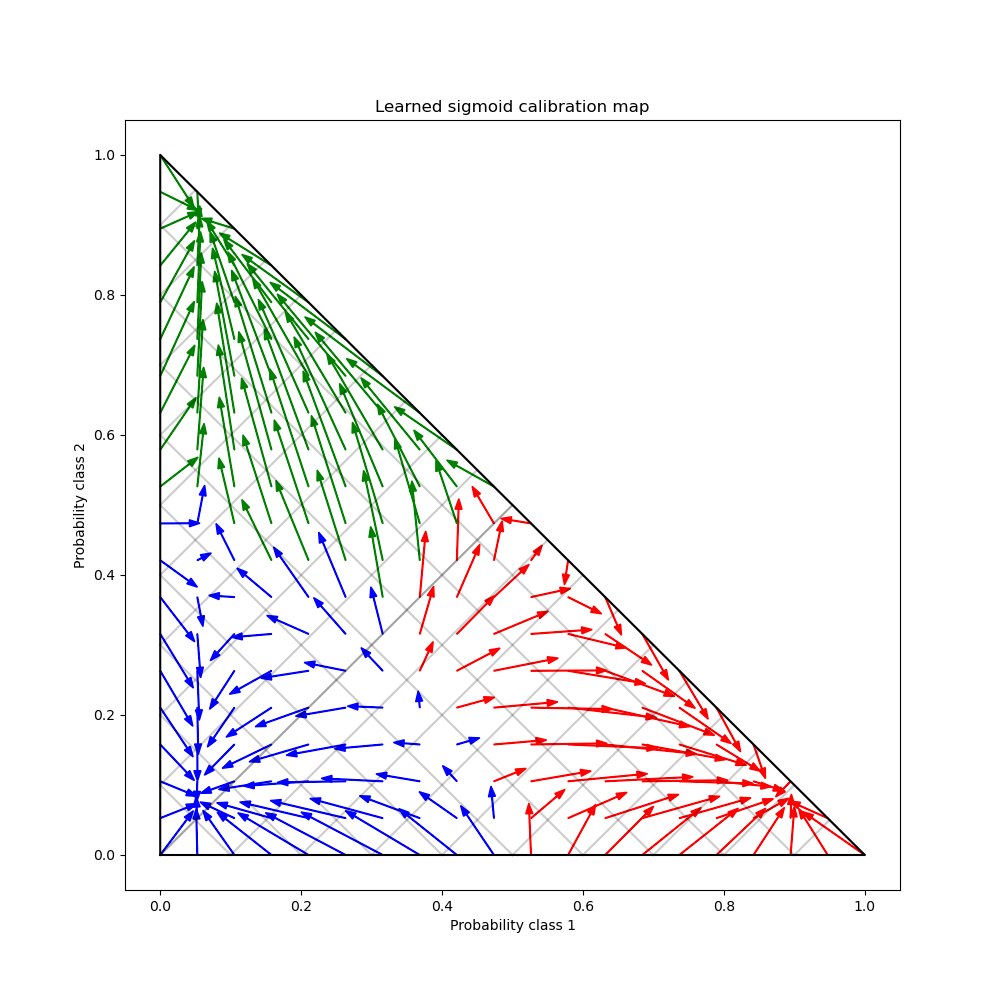
One can observe that, on average, the calibrator is pushing highly confident predictions away from the boundaries of the simplex while simultaneously moving uncertain predictions towards one of three modes, one for each class.
We can also observe that the mapping is not symmetric. Furthermore some arrows seems to cross class assignment boundaries: it means that some predicted classes change when taking the argmax over the predicted probabilities before and after calibration.
Let’s now repeat the above for various classifiers with different mis-calibration
profiles and the three calibration methods available in
CalibratedClassifierCV, namely, “sigmoid”, “isotonic”, and “temperature”.
Sigmoid and isotonic methods are implemented via a One-vs-Rest reduction to
binary calibration followed by sum-to-one normalization. Temperature scaling
fits a single temperature parameter on multinomial logits.
from collections import defaultdict

import pandas as pd

from sklearn.linear_model import LogisticRegression
from sklearn.naive_bayes import GaussianNB
from sklearn.pipeline import make_pipeline
from sklearn.preprocessing import PolynomialFeatures, SplineTransformer

base_classifiers = {
    "Random Forest (deep)": RandomForestClassifier(max_depth=8, random_state=42),
    "Random Forest (shallow)": RandomForestClassifier(max_depth=3, random_state=42),
    "Polynomial classifier (low reg)": make_pipeline(
        SplineTransformer(),
        PolynomialFeatures(interaction_only=True, include_bias=False),
        LogisticRegression(C=1e6, max_iter=1_000),
    ),
    "Polynomial classifier (high reg)": make_pipeline(
        SplineTransformer(),
        PolynomialFeatures(interaction_only=True, include_bias=False),
        LogisticRegression(C=1e-1, max_iter=1_000),
    ),
    "Gaussian Naive Bayes": GaussianNB(),
}

calibration_methods = ["temperature", "sigmoid", "isotonic"]
fig, axes = plt.subplots(
    nrows=len(base_classifiers),
    ncols=len(calibration_methods),
    figsize=(15, 5 * len(base_classifiers)),
    tight_layout=True,
)

scores = defaultdict(dict)

for classifier_idx, (name, base_clf) in enumerate(base_classifiers.items()):
    base_clf.fit(X_train, y_train)
    y_pred_uncal = base_clf.predict_proba(X_test)
    scores_for_classifier = scores[name]
    scores_for_classifier.update(
        {
            "Classifier": name,
            "Log-loss (original)": log_loss(y_test, y_pred_uncal),
            "Brier score (original)": brier_score_loss(y_test, y_pred_uncal),
        }
    )
    for method_idx, calibration_method in enumerate(calibration_methods):
        cal_clf = CalibratedClassifierCV(
            FrozenEstimator(base_clf), method=calibration_method
        )
        cal_clf.fit(X_cal, y_cal)
        y_pred_cal = cal_clf.predict_proba(X_test)
        plot_calibrator_map(
            cal_clf,
            title=f"{name} - {calibration_method}",
            annotate=False,
            ax=axes[classifier_idx, method_idx],
            display_legend=(classifier_idx == 0 and method_idx == 0),
        )
        scores_for_classifier.update(
            {
                f"Log-loss ({calibration_method})": log_loss(y_test, y_pred_cal),
                f"Brier score ({calibration_method})": brier_score_loss(
                    y_test, y_pred_cal
                ),
            }
        )
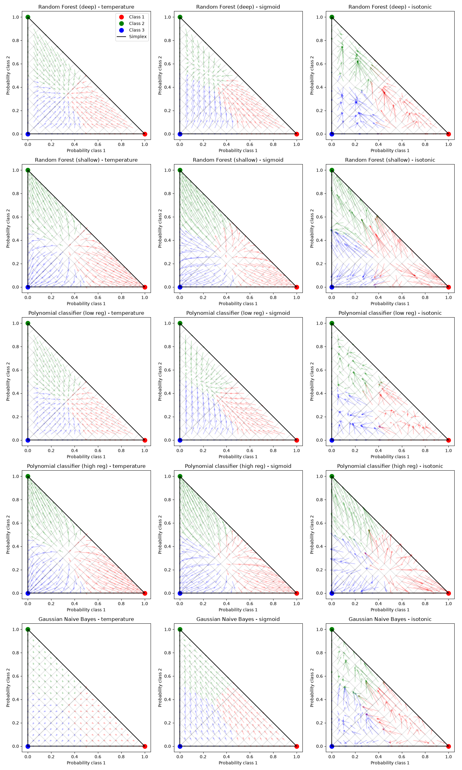
We observe the following:
Some estimators such as the highly regularized polynomial classifier and the shallow tree-based model tend to be under-confident by default and each kind of post-hoc calibration moves the predictions towards the edges or the corners of the simplex.
On the contrary, deep tree-based models and lowly regularized polynomial classifiers are over-confident by default and post-hoc calibration moves their predictions away from the edges of the simplex.
The Gaussian naive Bayes classifier receives the smallest corrections from the calibration: the arrows are short and the calibrated probabilities are close to the uncalibrated probabilities. This result is expected for this dataset as the data is generated from a class-wise mixture of Gaussian distributions with independent features. This could be very different if the data generation process did not match the assumptions of the naive Bayes model.
The sigmoid calibration method induces a smooth mapping of the uncalibrated probabilities to the calibrated probabilities. This smoothness is a result of parametric modeling of the calibration function with a small number of parameters and the use of the smooth logistic function.
The isotonic calibration method induces a piecewise constant mapping of the uncalibrated probabilities to the calibrated probabilities. To adapt to the multiclass setting, the One-vs-Rest strategy is used. As a result, the calibration maps show locally converging arrows to a finite number of points in the simplex. This effect is more pronounced with smaller calibration sets.
The temperature scaling method induces a smooth mapping that preserves the ranking of the predicted classes while adjusting their confidence.
Let us now consider the quantitative evaluation results of the available calibration methods:
reordered_columns = [
    "Classifier",
    "Log-loss (original)",
    "Log-loss (temperature)",
    "Log-loss (sigmoid)",
    "Log-loss (isotonic)",
    "Brier score (original)",
    "Brier score (temperature)",
    "Brier score (sigmoid)",
    "Brier score (isotonic)",
]
pd.DataFrame(scores.values())[reordered_columns].round(3)
The table above shows that the temperature and sigmoid calibration methods improve both the log-loss and the Brier score for all classifiers on this study. The results for the isotonic calibration method are more mixed, likely caused by the limited size of the calibration set.
To conclude, none of the calibration methods implemented in
CalibratedClassifierCV should be trusted blindly. It’s important to check
that post-hoc calibration is helpful from a quantitative point of view by
evaluating the classifier performance with and without calibration using
strictly proper scoring rules such as the log-loss or the Brier score.
plt.show()
Total running time of the script: (0 minutes 3.680 seconds)


Related examples
Analysis of the convergence of penalized logistic regression models