Note
Go to the end to download the full example code or to run this example in your browser via JupyterLite or Binder.
Gaussian Mixture Model Sine Curve#
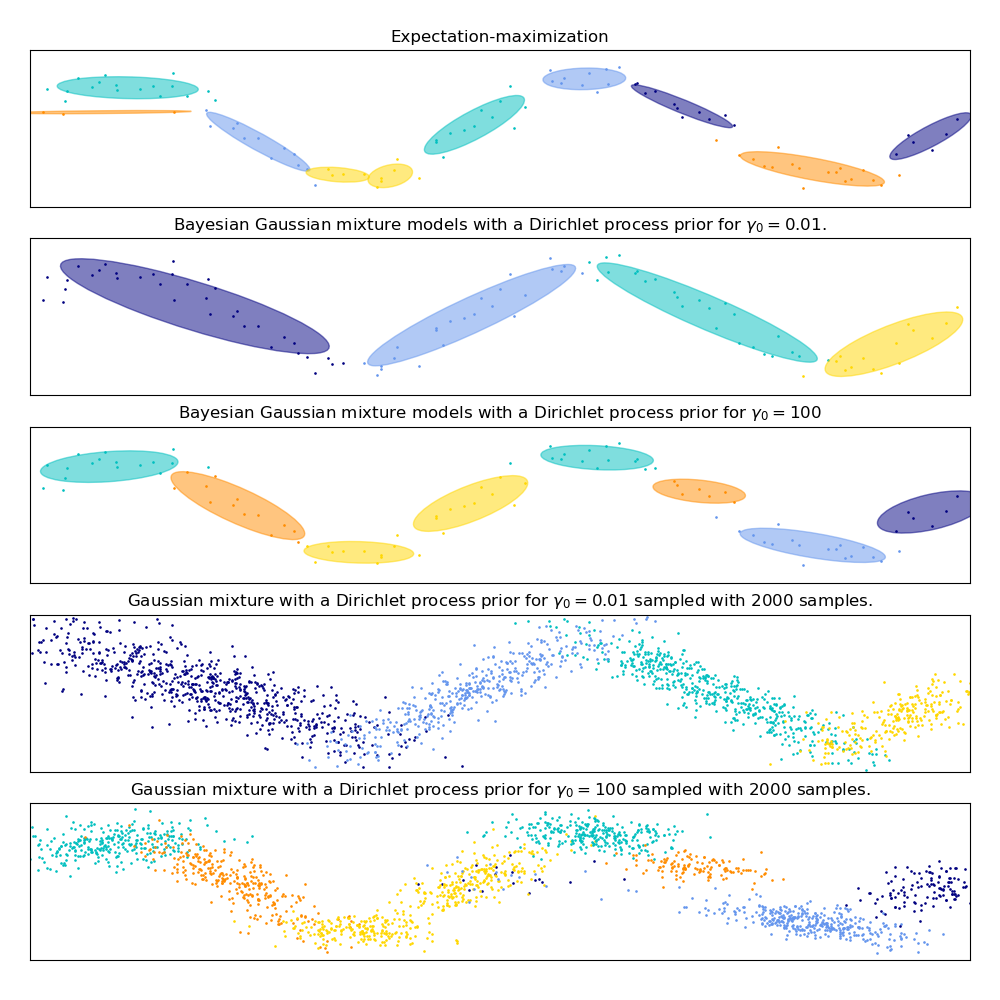
This example demonstrates the behavior of Gaussian mixture models fit on data that was not sampled from a mixture of Gaussian random variables. The dataset is formed by 100 points loosely spaced following a noisy sine curve. There is therefore no ground truth value for the number of Gaussian components.
The first model is a classical Gaussian Mixture Model with 10 components fit with the Expectation-Maximization algorithm.
The second model is a Bayesian Gaussian Mixture Model with a Dirichlet process prior fit with variational inference. The low value of the concentration prior makes the model favor a lower number of active components. This models “decides” to focus its modeling power on the big picture of the structure of the dataset: groups of points with alternating directions modeled by non-diagonal covariance matrices. Those alternating directions roughly capture the alternating nature of the original sine signal.
The third model is also a Bayesian Gaussian mixture model with a Dirichlet process prior but this time the value of the concentration prior is higher giving the model more liberty to model the fine-grained structure of the data. The result is a mixture with a larger number of active components that is similar to the first model where we arbitrarily decided to fix the number of components to 10.
Which model is the best is a matter of subjective judgment: do we want to favor models that only capture the big picture to summarize and explain most of the structure of the data while ignoring the details or do we prefer models that closely follow the high density regions of the signal?
The last two panels show how we can sample from the last two models. The resulting samples distributions do not look exactly like the original data distribution. The difference primarily stems from the approximation error we made by using a model that assumes that the data was generated by a finite number of Gaussian components instead of a continuous noisy sine curve.
# Authors: The scikit-learn developers
# SPDX-License-Identifier: BSD-3-Clause

import itertools

import matplotlib as mpl
import matplotlib.pyplot as plt
import numpy as np
from scipy import linalg

from sklearn import mixture

color_iter = itertools.cycle(["navy", "c", "cornflowerblue", "gold", "darkorange"])


def plot_results(X, Y, means, covariances, index, title):
    splot = plt.subplot(5, 1, 1 + index)
    for i, (mean, covar, color) in enumerate(zip(means, covariances, color_iter)):
        v, w = linalg.eigh(covar)
        v = 2.0 * np.sqrt(2.0) * np.sqrt(v)
        u = w[0] / linalg.norm(w[0])
        # as the DP will not use every component it has access to
        # unless it needs it, we shouldn't plot the redundant
        # components.
        if not np.any(Y == i):
            continue
        plt.scatter(X[Y == i, 0], X[Y == i, 1], 0.8, color=color)

        # Plot an ellipse to show the Gaussian component
        angle = np.arctan(u[1] / u[0])
        angle = 180.0 * angle / np.pi  # convert to degrees
        ell = mpl.patches.Ellipse(mean, v[0], v[1], angle=180.0 + angle, color=color)
        ell.set_clip_box(splot.bbox)
        ell.set_alpha(0.5)
        splot.add_artist(ell)

    plt.xlim(-6.0, 4.0 * np.pi - 6.0)
    plt.ylim(-5.0, 5.0)
    plt.title(title)
    plt.xticks(())
    plt.yticks(())


def plot_samples(X, Y, n_components, index, title):
    plt.subplot(5, 1, 4 + index)
    for i, color in zip(range(n_components), color_iter):
        # as the DP will not use every component it has access to
        # unless it needs it, we shouldn't plot the redundant
        # components.
        if not np.any(Y == i):
            continue
        plt.scatter(X[Y == i, 0], X[Y == i, 1], 0.8, color=color)

    plt.xlim(-6.0, 4.0 * np.pi - 6.0)
    plt.ylim(-5.0, 5.0)
    plt.title(title)
    plt.xticks(())
    plt.yticks(())


# Parameters
n_samples = 100

# Generate random sample following a sine curve
np.random.seed(0)
X = np.zeros((n_samples, 2))
step = 4.0 * np.pi / n_samples

for i in range(X.shape[0]):
    x = i * step - 6.0
    X[i, 0] = x + np.random.normal(0, 0.1)
    X[i, 1] = 3.0 * (np.sin(x) + np.random.normal(0, 0.2))

plt.figure(figsize=(10, 10))
plt.subplots_adjust(
    bottom=0.04, top=0.95, hspace=0.2, wspace=0.05, left=0.03, right=0.97
)

# Fit a Gaussian mixture with EM using ten components
gmm = mixture.GaussianMixture(
    n_components=10, covariance_type="full", max_iter=100
).fit(X)
plot_results(
    X, gmm.predict(X), gmm.means_, gmm.covariances_, 0, "Expectation-maximization"
)

dpgmm = mixture.BayesianGaussianMixture(
    n_components=10,
    covariance_type="full",
    weight_concentration_prior=1e-2,
    weight_concentration_prior_type="dirichlet_process",
    mean_precision_prior=1e-2,
    covariance_prior=1e0 * np.eye(2),
    init_params="random",
    max_iter=100,
    random_state=2,
).fit(X)
plot_results(
    X,
    dpgmm.predict(X),
    dpgmm.means_,
    dpgmm.covariances_,
    1,
    "Bayesian Gaussian mixture models with a Dirichlet process prior "
    r"for $\gamma_0=0.01$.",
)

X_s, y_s = dpgmm.sample(n_samples=2000)
plot_samples(
    X_s,
    y_s,
    dpgmm.n_components,
    0,
    "Gaussian mixture with a Dirichlet process prior "
    r"for $\gamma_0=0.01$ sampled with $2000$ samples.",
)

dpgmm = mixture.BayesianGaussianMixture(
    n_components=10,
    covariance_type="full",
    weight_concentration_prior=1e2,
    weight_concentration_prior_type="dirichlet_process",
    mean_precision_prior=1e-2,
    covariance_prior=1e0 * np.eye(2),
    init_params="kmeans",
    max_iter=100,
    random_state=2,
).fit(X)
plot_results(
    X,
    dpgmm.predict(X),
    dpgmm.means_,
    dpgmm.covariances_,
    2,
    "Bayesian Gaussian mixture models with a Dirichlet process prior "
    r"for $\gamma_0=100$",
)

X_s, y_s = dpgmm.sample(n_samples=2000)
plot_samples(
    X_s,
    y_s,
    dpgmm.n_components,
    1,
    "Gaussian mixture with a Dirichlet process prior "
    r"for $\gamma_0=100$ sampled with $2000$ samples.",
)

plt.show()
Total running time of the script: (0 minutes 0.465 seconds)
Related examples
Concentration Prior Type Analysis of Variation Bayesian Gaussian Mixture