Note
Go to the end to download the full example code or to run this example in your browser via JupyterLite or Binder.
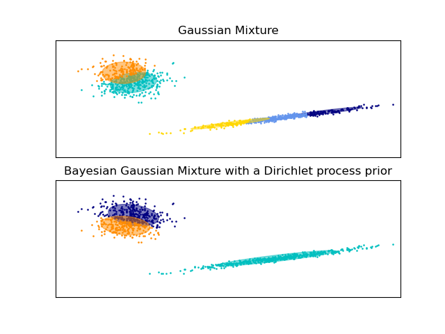
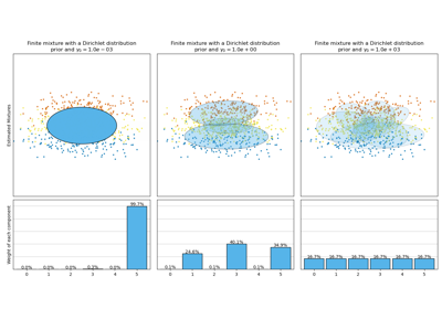
Gaussian Mixture Model Ellipsoids#
Plot the confidence ellipsoids of a mixture of two Gaussians
obtained with Expectation Maximisation (GaussianMixture class) and
Variational Inference (BayesianGaussianMixture class models with
a Dirichlet process prior).
Both models have access to five components with which to fit the data. Note that the Expectation Maximisation model will necessarily use all five components while the Variational Inference model will effectively only use as many as are needed for a good fit. Here we can see that the Expectation Maximisation model splits some components arbitrarily, because it is trying to fit too many components, while the Dirichlet Process model adapts it number of state automatically.
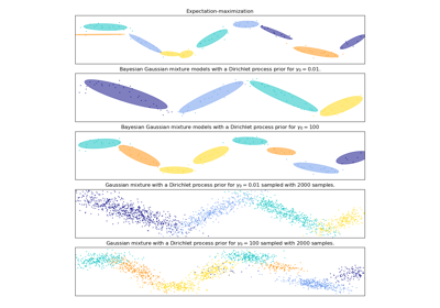
This example doesn’t show it, as we’re in a low-dimensional space, but another advantage of the Dirichlet process model is that it can fit full covariance matrices effectively even when there are less examples per cluster than there are dimensions in the data, due to regularization properties of the inference algorithm.
/home/circleci/project/sklearn/mixture/_base.py:293: ConvergenceWarning: Best performing initialization did not converge. Try different init parameters, or increase max_iter, tol, or check for degenerate data.
  warnings.warn(
# Authors: The scikit-learn developers
# SPDX-License-Identifier: BSD-3-Clause

import itertools

import matplotlib as mpl
import matplotlib.pyplot as plt
import numpy as np
from scipy import linalg

from sklearn import mixture

color_iter = itertools.cycle(["navy", "c", "cornflowerblue", "gold", "darkorange"])


def plot_results(X, Y_, means, covariances, index, title):
    splot = plt.subplot(2, 1, 1 + index)
    for i, (mean, covar, color) in enumerate(zip(means, covariances, color_iter)):
        v, w = linalg.eigh(covar)
        v = 2.0 * np.sqrt(2.0) * np.sqrt(v)
        u = w[0] / linalg.norm(w[0])
        # as the DP will not use every component it has access to
        # unless it needs it, we shouldn't plot the redundant
        # components.
        if not np.any(Y_ == i):
            continue
        plt.scatter(X[Y_ == i, 0], X[Y_ == i, 1], 0.8, color=color)

        # Plot an ellipse to show the Gaussian component
        angle = np.arctan(u[1] / u[0])
        angle = 180.0 * angle / np.pi  # convert to degrees
        ell = mpl.patches.Ellipse(mean, v[0], v[1], angle=180.0 + angle, color=color)
        ell.set_clip_box(splot.bbox)
        ell.set_alpha(0.5)
        splot.add_artist(ell)

    plt.xlim(-9.0, 5.0)
    plt.ylim(-3.0, 6.0)
    plt.xticks(())
    plt.yticks(())
    plt.title(title)


# Number of samples per component
n_samples = 500

# Generate random sample, two components
np.random.seed(0)
C = np.array([[0.0, -0.1], [1.7, 0.4]])
X = np.r_[
    np.dot(np.random.randn(n_samples, 2), C),
    0.7 * np.random.randn(n_samples, 2) + np.array([-6, 3]),
]

# Fit a Gaussian mixture with EM using five components
gmm = mixture.GaussianMixture(n_components=5, covariance_type="full").fit(X)
plot_results(X, gmm.predict(X), gmm.means_, gmm.covariances_, 0, "Gaussian Mixture")

# Fit a Dirichlet process Gaussian mixture using five components
dpgmm = mixture.BayesianGaussianMixture(n_components=5, covariance_type="full").fit(X)
plot_results(
    X,
    dpgmm.predict(X),
    dpgmm.means_,
    dpgmm.covariances_,
    1,
    "Bayesian Gaussian Mixture with a Dirichlet process prior",
)

plt.show()
Total running time of the script: (0 minutes 0.221 seconds)
Related examples
Concentration Prior Type Analysis of Variation Bayesian Gaussian Mixture