Blind source separation using FastICA

An example of estimating sources from noisy data.

Independent component analysis (ICA) is used to estimate sources given noisy measurements. Imagine 3 instruments playing simultaneously and 3 microphones recording the mixed signals. ICA is used to recover the sources ie. what is played by each instrument. Importantly, PCA fails at recovering our instruments since the related signals reflect non-Gaussian processes.

# Authors: The scikit-learn developers
# SPDX-License-Identifier: BSD-3-Clause

Generate sample data

import numpy as np
from scipy import signal

np.random.seed(0)
n_samples = 2000
time = np.linspace(0, 8, n_samples)

s1 = np.sin(2 * time)  # Signal 1 : sinusoidal signal
s2 = np.sign(np.sin(3 * time))  # Signal 2 : square signal
s3 = signal.sawtooth(2 * np.pi * time)  # Signal 3: saw tooth signal

S = np.c_[s1, s2, s3]
S += 0.2 * np.random.normal(size=S.shape)  # Add noise

S /= S.std(axis=0)  # Standardize data
# Mix data
A = np.array([[1, 1, 1], [0.5, 2, 1.0], [1.5, 1.0, 2.0]])  # Mixing matrix
X = np.dot(S, A.T)  # Generate observations

Fit ICA and PCA models

from sklearn.decomposition import PCA, FastICA

# Compute ICA
ica = FastICA(n_components=3, whiten="arbitrary-variance")
S_ = ica.fit_transform(X)  # Reconstruct signals
A_ = ica.mixing_  # Get estimated mixing matrix

# We can `prove` that the ICA model applies by reverting the unmixing.
assert np.allclose(X, np.dot(S_, A_.T) + ica.mean_)

# For comparison, compute PCA
pca = PCA(n_components=3)
H = pca.fit_transform(X)  # Reconstruct signals based on orthogonal components

Plot results

import matplotlib.pyplot as plt

plt.figure()

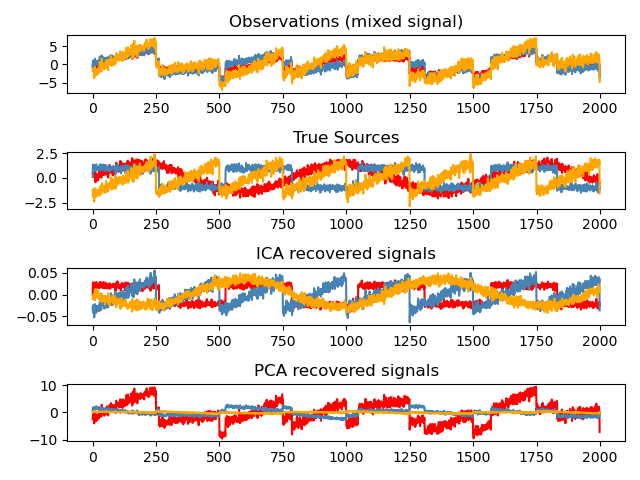
models = [X, S, S_, H]
names = [
    "Observations (mixed signal)",
    "True Sources",
    "ICA recovered signals",
    "PCA recovered signals",
]
colors = ["red", "steelblue", "orange"]

for ii, (model, name) in enumerate(zip(models, names), 1):
    plt.subplot(4, 1, ii)
    plt.title(name)
    for sig, color in zip(model.T, colors):
        plt.plot(sig, color=color)

plt.tight_layout()
plt.show()

Related examples

FastICA on 2D point clouds

FastICA on 2D point clouds

Orthogonal Matching Pursuit

Orthogonal Matching Pursuit

Comparison of kernel ridge and Gaussian process regression

Comparison of kernel ridge and Gaussian process regression

Sparse coding with a precomputed dictionary

Sparse coding with a precomputed dictionary