Ability of Gaussian process regression (GPR) to estimate data noise-level

This example shows the ability of the WhiteKernel to estimate the noise level in the data. Moreover, we show the importance of kernel hyperparameters initialization.

# Authors: The scikit-learn developers
# SPDX-License-Identifier: BSD-3-Clause

Data generation

We will work in a setting where X will contain a single feature. We create a function that will generate the target to be predicted. We will add an option to add some noise to the generated target.

import numpy as np


def target_generator(X, add_noise=False):
    target = 0.5 + np.sin(3 * X)
    if add_noise:
        rng = np.random.RandomState(1)
        target += rng.normal(0, 0.3, size=target.shape)
    return target.squeeze()

Let’s have a look to the target generator where we will not add any noise to observe the signal that we would like to predict.

X = np.linspace(0, 5, num=80).reshape(-1, 1)
y = target_generator(X, add_noise=False)

import matplotlib.pyplot as plt

plt.plot(X, y, label="Expected signal")
plt.legend()
plt.xlabel("X")
_ = plt.ylabel("y")

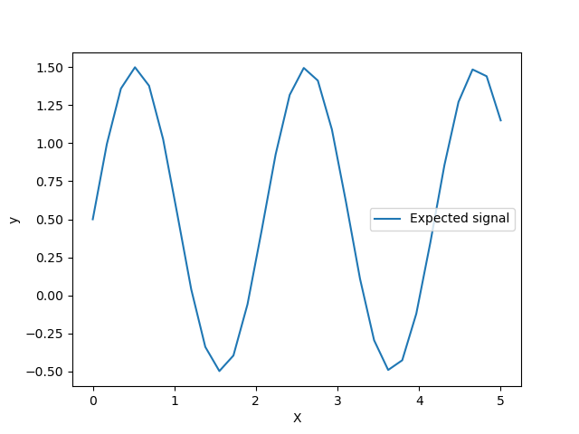
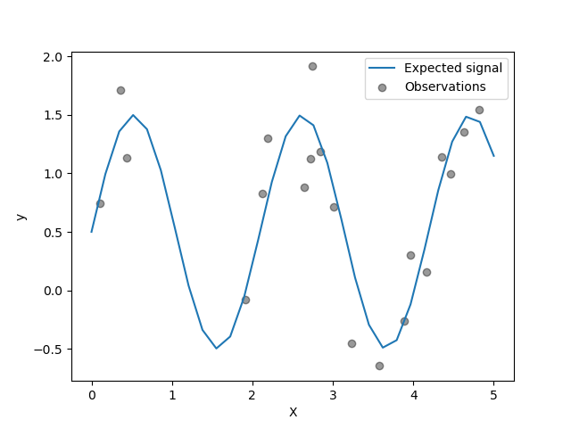
The target is transforming the input X using a sine function. Now, we will generate few noisy training samples. To illustrate the noise level, we will plot the true signal together with the noisy training samples.

rng = np.random.RandomState(0)
X_train = rng.uniform(0, 5, size=20).reshape(-1, 1)
y_train = target_generator(X_train, add_noise=True)

plt.plot(X, y, label="Expected signal")
plt.scatter(
    x=X_train[:, 0],
    y=y_train,
    color="black",
    alpha=0.4,
    label="Observations",
)
plt.legend()
plt.xlabel("X")
_ = plt.ylabel("y")

Optimisation of kernel hyperparameters in GPR

Now, we will create a GaussianProcessRegressor using an additive kernel adding a RBF and WhiteKernel kernels. The WhiteKernel is a kernel that will able to estimate the amount of noise present in the data while the RBF will serve at fitting the non-linearity between the data and the target.

However, we will show that the hyperparameter space contains several local minima. It will highlights the importance of initial hyperparameter values.

We will create a model using a kernel with a high noise level and a large length scale, which will explain all variations in the data by noise.

from sklearn.gaussian_process import GaussianProcessRegressor
from sklearn.gaussian_process.kernels import RBF, WhiteKernel

kernel = 1.0 * RBF(length_scale=1e1, length_scale_bounds=(1e-2, 1e3)) + WhiteKernel(
    noise_level=1, noise_level_bounds=(1e-10, 1e1)
)
gpr = GaussianProcessRegressor(kernel=kernel, alpha=0.0)
gpr.fit(X_train, y_train)
y_mean, y_std = gpr.predict(X, return_std=True)

/home/circleci/project/sklearn/gaussian_process/kernels.py:452: ConvergenceWarning:

The optimal value found for dimension 0 of parameter k1__k2__length_scale is close to the specified upper bound 1000.0. Increasing the bound and calling fit again may find a better value.

plt.plot(X, y, label="Expected signal")
plt.scatter(x=X_train[:, 0], y=y_train, color="black", alpha=0.4, label="Observations")
plt.errorbar(X, y_mean, y_std, label="Posterior mean ± std")
plt.legend()
plt.xlabel("X")
plt.ylabel("y")
_ = plt.title(
    (
        f"Initial: {kernel}\nOptimum: {gpr.kernel_}\nLog-Marginal-Likelihood: "
        f"{gpr.log_marginal_likelihood(gpr.kernel_.theta)}"
    ),
    fontsize=8,
)

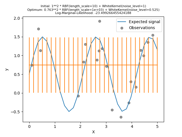
We see that the optimum kernel found still has a high noise level and an even larger length scale. The length scale reaches the maximum bound that we allowed for this parameter and we got a warning as a result.

More importantly, we observe that the model does not provide useful predictions: the mean prediction seems to be constant: it does not follow the expected noise-free signal.

Now, we will initialize the RBF with a larger length_scale initial value and the WhiteKernel with a smaller initial noise level lower while keeping the parameter bounds unchanged.

kernel = 1.0 * RBF(length_scale=1e-1, length_scale_bounds=(1e-2, 1e3)) + WhiteKernel(
    noise_level=1e-2, noise_level_bounds=(1e-10, 1e1)
)
gpr = GaussianProcessRegressor(kernel=kernel, alpha=0.0)
gpr.fit(X_train, y_train)
y_mean, y_std = gpr.predict(X, return_std=True)

plt.plot(X, y, label="Expected signal")
plt.scatter(x=X_train[:, 0], y=y_train, color="black", alpha=0.4, label="Observations")
plt.errorbar(X, y_mean, y_std, label="Posterior mean ± std")
plt.legend()
plt.xlabel("X")
plt.ylabel("y")
_ = plt.title(
    (
        f"Initial: {kernel}\nOptimum: {gpr.kernel_}\nLog-Marginal-Likelihood: "
        f"{gpr.log_marginal_likelihood(gpr.kernel_.theta)}"
    ),
    fontsize=8,
)

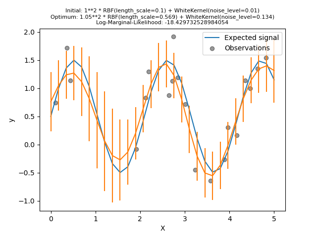
First, we see that the model’s predictions are more precise than the previous model’s: this new model is able to estimate the noise-free functional relationship.

Looking at the kernel hyperparameters, we see that the best combination found has a smaller noise level and shorter length scale than the first model.

We can inspect the negative Log-Marginal-Likelihood (LML) of GaussianProcessRegressor for different hyperparameters to get a sense of the local minima.

from matplotlib.colors import LogNorm

length_scale = np.logspace(-2, 4, num=80)
noise_level = np.logspace(-2, 1, num=80)
length_scale_grid, noise_level_grid = np.meshgrid(length_scale, noise_level)

log_marginal_likelihood = [
    gpr.log_marginal_likelihood(theta=np.log([0.36, scale, noise]))
    for scale, noise in zip(length_scale_grid.ravel(), noise_level_grid.ravel())
]
log_marginal_likelihood = np.reshape(log_marginal_likelihood, noise_level_grid.shape)

vmin, vmax = (-log_marginal_likelihood).min(), 50
level = np.around(np.logspace(np.log10(vmin), np.log10(vmax), num=20), decimals=1)
plt.contour(
    length_scale_grid,
    noise_level_grid,
    -log_marginal_likelihood,
    levels=level,
    norm=LogNorm(vmin=vmin, vmax=vmax),
)
plt.colorbar()
plt.xscale("log")
plt.yscale("log")
plt.xlabel("Length-scale")
plt.ylabel("Noise-level")
plt.title("Negative log-marginal-likelihood")
plt.show()

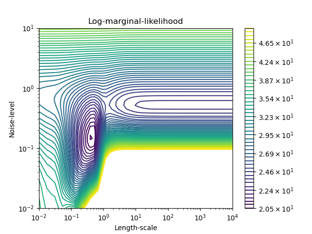
We see that there are two local minima that correspond to the combination of hyperparameters previously found. Depending on the initial values for the hyperparameters, the gradient-based optimization might or might not converge to the best model. It is thus important to repeat the optimization several times for different initializations. This can be done by setting the n_restarts_optimizer parameter of the GaussianProcessRegressor class.

Let’s try again to fit our model with the bad initial values but this time with 10 random restarts.

kernel = 1.0 * RBF(length_scale=1e1, length_scale_bounds=(1e-2, 1e3)) + WhiteKernel(
    noise_level=1, noise_level_bounds=(1e-10, 1e1)
)
gpr = GaussianProcessRegressor(
    kernel=kernel, alpha=0.0, n_restarts_optimizer=10, random_state=0
)
gpr.fit(X_train, y_train)
y_mean, y_std = gpr.predict(X, return_std=True)

plt.plot(X, y, label="Expected signal")
plt.scatter(x=X_train[:, 0], y=y_train, color="black", alpha=0.4, label="Observations")
plt.errorbar(X, y_mean, y_std, label="Posterior mean ± std")
plt.legend()
plt.xlabel("X")
plt.ylabel("y")
_ = plt.title(
    (
        f"Initial: {kernel}\nOptimum: {gpr.kernel_}\nLog-Marginal-Likelihood: "
        f"{gpr.log_marginal_likelihood(gpr.kernel_.theta)}"
    ),
    fontsize=8,
)

As we hoped, random restarts allow the optimization to find the best set of hyperparameters despite the bad initial values.

Related examples

Illustration of prior and posterior Gaussian process for different kernels

Illustration of prior and posterior Gaussian process for different kernels

Gaussian Processes regression: basic introductory example

Gaussian Processes regression: basic introductory example

Probabilistic predictions with Gaussian process classification (GPC)

Probabilistic predictions with Gaussian process classification (GPC)

Comparison of kernel ridge and Gaussian process regression

Comparison of kernel ridge and Gaussian process regression