Note
Go to the end to download the full example code or to run this example in your browser via JupyterLite or Binder.
Forecasting of CO2 level on Mona Loa dataset using Gaussian process regression (GPR)#
This example is based on Section 5.4.3 of “Gaussian Processes for Machine Learning” [1]. It illustrates an example of complex kernel engineering and hyperparameter optimization using gradient ascent on the log-marginal-likelihood. The data consists of the monthly average atmospheric CO2 concentrations (in parts per million by volume (ppm)) collected at the Mauna Loa Observatory in Hawaii, between 1958 and 2001. The objective is to model the CO2 concentration as a function of the time \(t\) and extrapolate for years after 2001.
References
# Authors: The scikit-learn developers
# SPDX-License-Identifier: BSD-3-Clause
Build the dataset#
We will derive a dataset from the Mauna Loa Observatory that collected air
samples. We are interested in estimating the concentration of CO2 and
extrapolate it for further years. First, we load the original dataset available
in OpenML as a pandas dataframe. This will be replaced with Polars
once fetch_openml adds a native support for it.
from sklearn.datasets import fetch_openml

co2 = fetch_openml(data_id=41187, as_frame=True)
co2.frame.head()
First, we process the original dataframe to create a date column and select it along with the CO2 column.
import polars as pl

co2_data = pl.DataFrame(co2.frame[["year", "month", "day", "co2"]]).select(
    pl.date("year", "month", "day"), "co2"
)
co2_data.head()
co2_data["date"].min(), co2_data["date"].max()
(datetime.date(1958, 3, 29), datetime.date(2001, 12, 29))
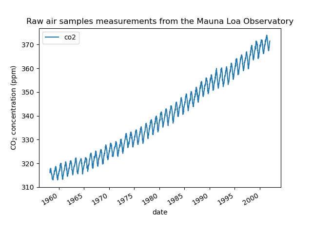
We see that we get CO2 concentration for some days from March, 1958 to December, 2001. We can plot the raw information to have a better understanding.
import matplotlib.pyplot as plt

plt.plot(co2_data["date"], co2_data["co2"])
plt.xlabel("date")
plt.ylabel("CO$_2$ concentration (ppm)")
_ = plt.title("Raw air samples measurements from the Mauna Loa Observatory")
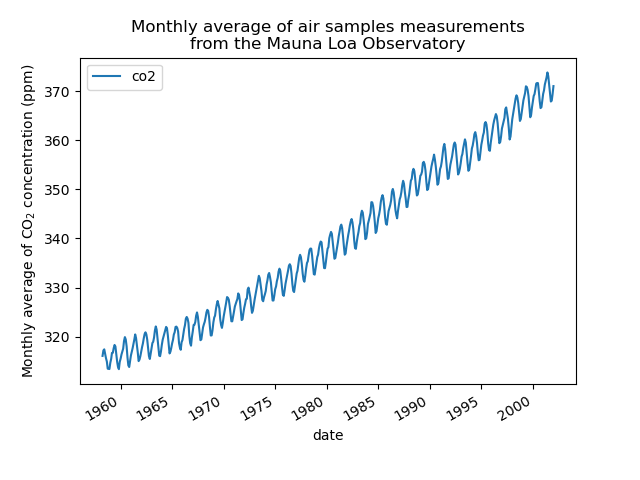
We will preprocess the dataset by taking a monthly average and drop months for which no measurements were collected. Such a processing will have a smoothing effect on the data.
co2_data = (
    co2_data.sort(by="date")
    .group_by_dynamic("date", every="1mo")
    .agg(pl.col("co2").mean())
    .drop_nulls()
)
plt.plot(co2_data["date"], co2_data["co2"])
plt.xlabel("date")
plt.ylabel("Monthly average of CO$_2$ concentration (ppm)")
_ = plt.title(
    "Monthly average of air samples measurements\nfrom the Mauna Loa Observatory"
)
The idea in this example will be to predict the CO2 concentration in function of the date. We are as well interested in extrapolating for upcoming year after 2001.
As a first step, we will divide the data and the target to estimate. The data being a date, we will convert it into a numeric.
X = co2_data.select(
    pl.col("date").dt.year() + pl.col("date").dt.month() / 12
).to_numpy()
y = co2_data["co2"].to_numpy()
Design the proper kernel#
To design the kernel to use with our Gaussian process, we can make some assumption regarding the data at hand. We observe that they have several characteristics: we see a long term rising trend, a pronounced seasonal variation and some smaller irregularities. We can use different appropriate kernel that would capture these features.
First, the long term rising trend could be fitted using a radial basis function (RBF) kernel with a large length-scale parameter. The RBF kernel with a large length-scale enforces this component to be smooth. A trending increase is not enforced as to give a degree of freedom to our model. The specific length-scale and the amplitude are free hyperparameters.
The seasonal variation is explained by the periodic exponential sine squared kernel with a fixed periodicity of 1 year. The length-scale of this periodic component, controlling its smoothness, is a free parameter. In order to allow decaying away from exact periodicity, the product with an RBF kernel is taken. The length-scale of this RBF component controls the decay time and is a further free parameter. This type of kernel is also known as locally periodic kernel.
from sklearn.gaussian_process.kernels import ExpSineSquared

seasonal_kernel = (
    2.0**2
    * RBF(length_scale=100.0)
    * ExpSineSquared(length_scale=1.0, periodicity=1.0, periodicity_bounds="fixed")
)
The small irregularities are to be explained by a rational quadratic kernel component, whose length-scale and alpha parameter, which quantifies the diffuseness of the length-scales, are to be determined. A rational quadratic kernel is equivalent to an RBF kernel with several length-scale and will better accommodate the different irregularities.
from sklearn.gaussian_process.kernels import RationalQuadratic

irregularities_kernel = 0.5**2 * RationalQuadratic(length_scale=1.0, alpha=1.0)
Finally, the noise in the dataset can be accounted with a kernel consisting of an RBF kernel contribution, which shall explain the correlated noise components such as local weather phenomena, and a white kernel contribution for the white noise. The relative amplitudes and the RBF’s length scale are further free parameters.
from sklearn.gaussian_process.kernels import WhiteKernel

noise_kernel = 0.1**2 * RBF(length_scale=0.1) + WhiteKernel(
    noise_level=0.1**2, noise_level_bounds=(1e-5, 1e5)
)
Thus, our final kernel is an addition of all previous kernel.
co2_kernel = (
    long_term_trend_kernel + seasonal_kernel + irregularities_kernel + noise_kernel
)
co2_kernel
50**2 * RBF(length_scale=50) + 2**2 * RBF(length_scale=100) * ExpSineSquared(length_scale=1, periodicity=1) + 0.5**2 * RationalQuadratic(alpha=1, length_scale=1) + 0.1**2 * RBF(length_scale=0.1) + WhiteKernel(noise_level=0.01)
Model fitting and extrapolation#
Now, we are ready to use a Gaussian process regressor and fit the available
data. To follow the example from the literature, we will subtract the mean
from the target. We could have used normalize_y=True. However, doing so
would have also scaled the target (dividing y by its standard deviation).
Thus, the hyperparameters of the different kernel would have had different
meaning since they would not have been expressed in ppm.
from sklearn.gaussian_process import GaussianProcessRegressor

y_mean = y.mean()
gaussian_process = GaussianProcessRegressor(kernel=co2_kernel, normalize_y=False)
gaussian_process.fit(X, y - y_mean)
Now, we will use the Gaussian process to predict on:
training data to inspect the goodness of fit;
future data to see the extrapolation done by the model.
Thus, we create synthetic data from 1958 to the current month. In addition, we need to add the subtracted mean computed during training.
import datetime

import numpy as np

today = datetime.datetime.now()
current_month = today.year + today.month / 12
X_test = np.linspace(start=1958, stop=current_month, num=1_000).reshape(-1, 1)
mean_y_pred, std_y_pred = gaussian_process.predict(X_test, return_std=True)
mean_y_pred += y_mean
plt.plot(X, y, color="black", linestyle="dashed", label="Measurements")
plt.plot(X_test, mean_y_pred, color="tab:blue", alpha=0.4, label="Gaussian process")
plt.fill_between(
    X_test.ravel(),
    mean_y_pred - std_y_pred,
    mean_y_pred + std_y_pred,
    color="tab:blue",
    alpha=0.2,
)
plt.legend()
plt.xlabel("Year")
plt.ylabel("Monthly average of CO$_2$ concentration (ppm)")
_ = plt.title(
    "Monthly average of air samples measurements\nfrom the Mauna Loa Observatory"
)
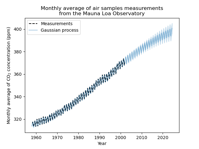
Our fitted model is capable to fit previous data properly and extrapolate to future year with confidence.
Interpretation of kernel hyperparameters#
Now, we can have a look at the hyperparameters of the kernel.
gaussian_process.kernel_
44.8**2 * RBF(length_scale=51.6) + 2.64**2 * RBF(length_scale=91.5) * ExpSineSquared(length_scale=1.48, periodicity=1) + 0.536**2 * RationalQuadratic(alpha=2.89, length_scale=0.968) + 0.188**2 * RBF(length_scale=0.122) + WhiteKernel(noise_level=0.0367)
Thus, most of the target signal, with the mean subtracted, is explained by a long-term rising trend for ~45 ppm and a length-scale of ~52 years. The periodic component has an amplitude of ~2.6ppm, a decay time of ~90 years and a length-scale of ~1.5. The long decay time indicates that we have a component very close to a seasonal periodicity. The correlated noise has an amplitude of ~0.2 ppm with a length scale of ~0.12 years and a white-noise contribution of ~0.04 ppm. Thus, the overall noise level is very small, indicating that the data can be very well explained by the model.
Total running time of the script: (0 minutes 4.136 seconds)
Related examples

Gaussian Processes regression: basic introductory example
Ability of Gaussian process regression (GPR) to estimate data noise-level
Comparison of kernel ridge and Gaussian process regression
Gaussian process classification (GPC) on iris dataset
