Note
Go to the end to download the full example code or to run this example in your browser via JupyterLite or Binder.
Hierarchical clustering with and without structure#
This example demonstrates hierarchical clustering with and without connectivity constraints. It shows the effect of imposing a connectivity graph to capture local structure in the data. Without connectivity constraints, the clustering is based purely on distance, while with constraints, the clustering respects local structure.
For more information, see Hierarchical clustering.
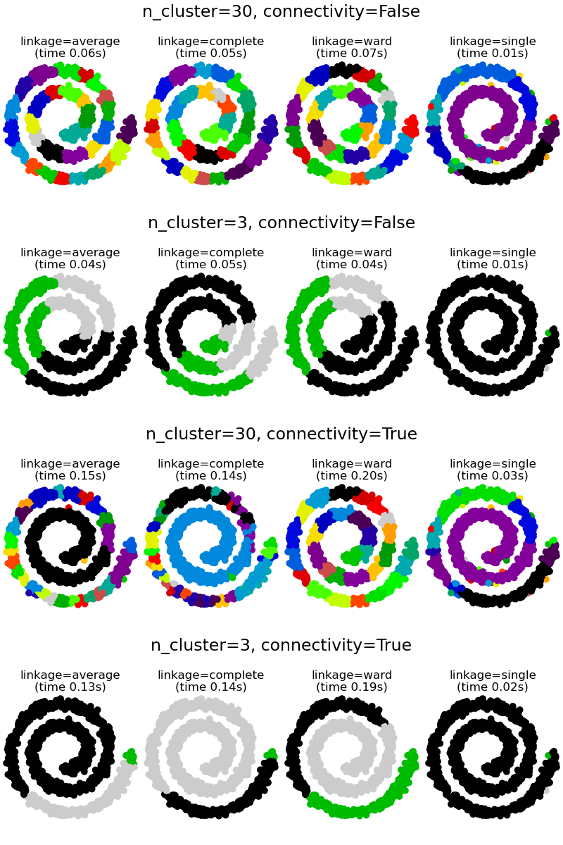
There are two advantages of imposing connectivity. First, clustering with sparse connectivity matrices is faster in general.
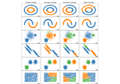
Second, when using a connectivity matrix, single, average and complete
linkage are unstable and tend to create a few clusters that grow very
quickly. Indeed, average and complete linkage fight this percolation behavior
by considering all the distances between two clusters when merging them
(while single linkage exaggerates the behaviour by considering only the
shortest distance between clusters). The connectivity graph breaks this
mechanism for average and complete linkage, making them resemble the more
brittle single linkage. This effect is more pronounced for very sparse graphs
(try decreasing the number of neighbors in kneighbors_graph) and with
complete linkage. In particular, having a very small number of neighbors in
the graph, imposes a geometry that is close to that of single linkage,
which is well known to have this percolation instability.
The effect of imposing connectivity is illustrated on two different but similar datasets which show a spiral structure. In the first example we build a Swiss roll dataset and run hierarchical clustering on the position of the data. Here, we compare unstructured Ward clustering with a structured variant that enforces k-Nearest Neighbors connectivity. In the second example we include the effects of applying a such a connectivity graph to single, average and complete linkage.
# Authors: The scikit-learn developers
# SPDX-License-Identifier: BSD-3-Clause
Generate the Swiss Roll dataset.#
import time

from sklearn.cluster import AgglomerativeClustering
from sklearn.datasets import make_swiss_roll

n_samples = 1500
noise = 0.05
X1, _ = make_swiss_roll(n_samples, noise=noise)
X1[:, 1] *= 0.5  # Make the roll thinner
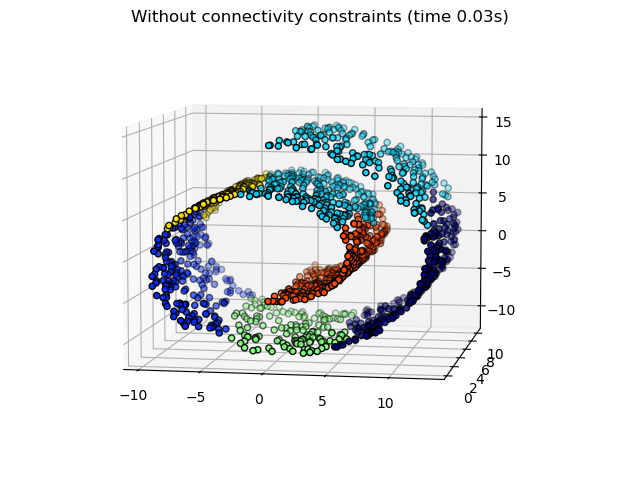
Compute clustering without connectivity constraints#
print("Compute unstructured hierarchical clustering...")
st = time.time()
ward_unstructured = AgglomerativeClustering(n_clusters=6, linkage="ward").fit(X1)
elapsed_time_unstructured = time.time() - st
label_unstructured = ward_unstructured.labels_
print(f"Elapsed time: {elapsed_time_unstructured:.2f}s")
print(f"Number of points: {label_unstructured.size}")
Compute unstructured hierarchical clustering...
Elapsed time: 0.03s
Number of points: 1500
Plot unstructured clustering result
import matplotlib.pyplot as plt
import numpy as np

fig1 = plt.figure()
ax1 = fig1.add_subplot(111, projection="3d", elev=7, azim=-80)
ax1.set_position([0, 0, 0.95, 1])
for l in np.unique(label_unstructured):
    ax1.scatter(
        X1[label_unstructured == l, 0],
        X1[label_unstructured == l, 1],
        X1[label_unstructured == l, 2],
        color=plt.cm.jet(float(l) / np.max(label_unstructured + 1)),
        s=20,
        edgecolor="k",
    )
_ = fig1.suptitle(
    f"Without connectivity constraints (time {elapsed_time_unstructured:.2f}s)"
)
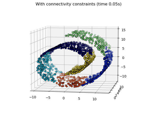
Compute clustering with connectivity constraints#
from sklearn.neighbors import kneighbors_graph

connectivity = kneighbors_graph(X1, n_neighbors=10, include_self=False)

print("Compute structured hierarchical clustering...")
st = time.time()
ward_structured = AgglomerativeClustering(
    n_clusters=6, connectivity=connectivity, linkage="ward"
).fit(X1)
elapsed_time_structured = time.time() - st
label_structured = ward_structured.labels_
print(f"Elapsed time: {elapsed_time_structured:.2f}s")
print(f"Number of points: {label_structured.size}")
Compute structured hierarchical clustering...
Elapsed time: 0.06s
Number of points: 1500
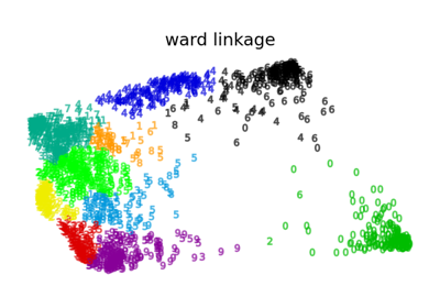
Plot structured clustering result
fig2 = plt.figure()
ax2 = fig2.add_subplot(111, projection="3d", elev=7, azim=-80)
ax2.set_position([0, 0, 0.95, 1])
for l in np.unique(label_structured):
    ax2.scatter(
        X1[label_structured == l, 0],
        X1[label_structured == l, 1],
        X1[label_structured == l, 2],
        color=plt.cm.jet(float(l) / np.max(label_structured + 1)),
        s=20,
        edgecolor="k",
    )
_ = fig2.suptitle(
    f"With connectivity constraints (time {elapsed_time_structured:.2f}s)"
)
Generate 2D spiral dataset.#
n_samples = 1500
np.random.seed(0)
t = 1.5 * np.pi * (1 + 3 * np.random.rand(1, n_samples))
x = t * np.cos(t)
y = t * np.sin(t)

X2 = np.concatenate((x, y))
X2 += 0.7 * np.random.randn(2, n_samples)
X2 = X2.T
Capture local connectivity using a graph#
Larger number of neighbors will give more homogeneous clusters to the cost of computation time. A very large number of neighbors gives more evenly distributed cluster sizes, but may not impose the local manifold structure of the data.
knn_graph = kneighbors_graph(X2, 30, include_self=False)
Plot clustering with and without structure#
fig3 = plt.figure(figsize=(8, 12))
subfigs = fig3.subfigures(4, 1)
params = [
    (None, 30),
    (None, 3),
    (knn_graph, 30),
    (knn_graph, 3),
]

for subfig, (connectivity, n_clusters) in zip(subfigs, params):
    axs = subfig.subplots(1, 4, sharey=True)
    for index, linkage in enumerate(("average", "complete", "ward", "single")):
        model = AgglomerativeClustering(
            linkage=linkage, connectivity=connectivity, n_clusters=n_clusters
        )
        t0 = time.time()
        model.fit(X2)
        elapsed_time = time.time() - t0
        axs[index].scatter(
            X2[:, 0], X2[:, 1], c=model.labels_, cmap=plt.cm.nipy_spectral
        )
        axs[index].set_title(
            "linkage=%s\n(time %.2fs)" % (linkage, elapsed_time),
            fontdict=dict(verticalalignment="top"),
        )
        axs[index].set_aspect("equal")
        axs[index].axis("off")

        subfig.subplots_adjust(bottom=0, top=0.83, wspace=0, left=0, right=1)
        subfig.suptitle(
            "n_cluster=%i, connectivity=%r" % (n_clusters, connectivity is not None),
            size=17,
        )

plt.show()
Total running time of the script: (0 minutes 2.086 seconds)
Related examples
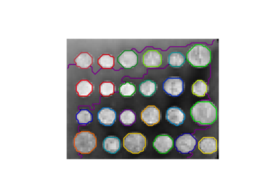
A demo of structured Ward hierarchical clustering on an image of coins
Comparing different hierarchical linkage methods on toy datasets
Various Agglomerative Clustering on a 2D embedding of digits
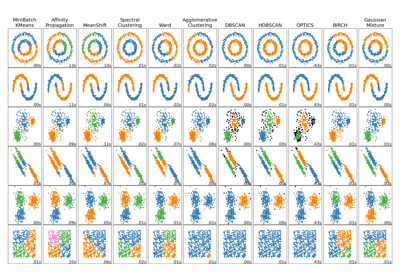
Comparing different clustering algorithms on toy datasets