Note
Go to the end to download the full example code or to run this example in your browser via JupyterLite or Binder.
Comparing Linear Bayesian Regressors#
This example compares two different bayesian regressors:
In the first part, we use an Ordinary Least Squares (OLS) model as a baseline for comparing the models’ coefficients with respect to the true coefficients. Thereafter, we show that the estimation of such models is done by iteratively maximizing the marginal log-likelihood of the observations.
In the last section we plot predictions and uncertainties for the ARD and the
Bayesian Ridge regressions using a polynomial feature expansion to fit a
non-linear relationship between X and y.
# Authors: The scikit-learn developers
# SPDX-License-Identifier: BSD-3-Clause
Models robustness to recover the ground truth weights#
Generate synthetic dataset#
We generate a dataset where X and y are linearly linked: 10 of the
features of X will be used to generate y. The other features are not
useful at predicting y. In addition, we generate a dataset where n_samples
== n_features. Such a setting is challenging for an OLS model and leads
potentially to arbitrary large weights. Having a prior on the weights and a
penalty alleviates the problem. Finally, gaussian noise is added.
from sklearn.datasets import make_regression

X, y, true_weights = make_regression(
    n_samples=100,
    n_features=100,
    n_informative=10,
    noise=8,
    coef=True,
    random_state=42,
)
Fit the regressors#
We now fit both Bayesian models and the OLS to later compare the models’ coefficients.
import pandas as pd

from sklearn.linear_model import ARDRegression, BayesianRidge, LinearRegression

olr = LinearRegression().fit(X, y)
brr = BayesianRidge(compute_score=True, max_iter=30).fit(X, y)
ard = ARDRegression(compute_score=True, max_iter=30).fit(X, y)
df = pd.DataFrame(
    {
        "Weights of true generative process": true_weights,
        "ARDRegression": ard.coef_,
        "BayesianRidge": brr.coef_,
        "LinearRegression": olr.coef_,
    }
)
Plot the true and estimated coefficients#
Now we compare the coefficients of each model with the weights of the true generative model.
import matplotlib.pyplot as plt
import seaborn as sns
from matplotlib.colors import SymLogNorm

plt.figure(figsize=(10, 6))
ax = sns.heatmap(
    df.T,
    norm=SymLogNorm(linthresh=10e-4, vmin=-80, vmax=80),
    cbar_kws={"label": "coefficients' values"},
    cmap="seismic_r",
)
plt.ylabel("linear model")
plt.xlabel("coefficients")
plt.tight_layout(rect=(0, 0, 1, 0.95))
_ = plt.title("Models' coefficients")
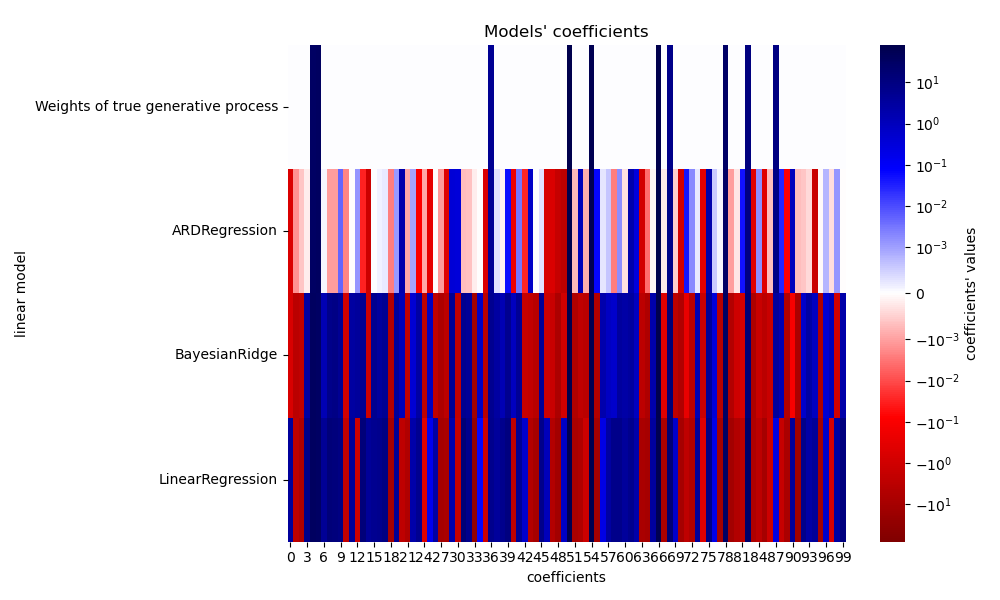
Due to the added noise, none of the models recover the true weights. Indeed, all models always have more than 10 non-zero coefficients. Compared to the OLS estimator, the coefficients using a Bayesian Ridge regression are slightly shifted toward zero, which stabilises them. The ARD regression provides a sparser solution: some of the non-informative coefficients are set exactly to zero, while shifting others closer to zero. Some non-informative coefficients are still present and retain large values.
Plot the marginal log-likelihood#
import numpy as np

ard_scores = -np.array(ard.scores_)
brr_scores = -np.array(brr.scores_)
plt.plot(ard_scores, color="navy", label="ARD")
plt.plot(brr_scores, color="red", label="BayesianRidge")
plt.ylabel("Log-likelihood")
plt.xlabel("Iterations")
plt.xlim(1, 30)
plt.legend()
_ = plt.title("Models log-likelihood")
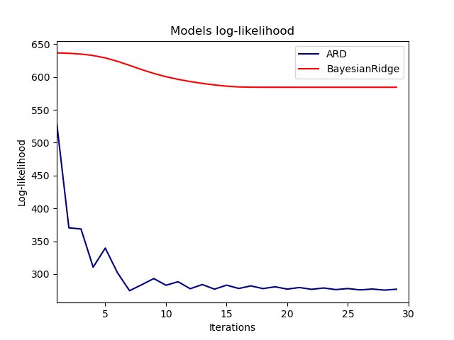
Indeed, both models minimize the log-likelihood up to an arbitrary cutoff
defined by the max_iter parameter.
Bayesian regressions with polynomial feature expansion#
Generate synthetic dataset#
We create a target that is a non-linear function of the input feature. Noise following a standard uniform distribution is added.
from sklearn.pipeline import make_pipeline
from sklearn.preprocessing import PolynomialFeatures, StandardScaler

rng = np.random.RandomState(0)
n_samples = 110

# sort the data to make plotting easier later
X = np.sort(-10 * rng.rand(n_samples) + 10)
noise = rng.normal(0, 1, n_samples) * 1.35
y = np.sqrt(X) * np.sin(X) + noise
full_data = pd.DataFrame({"input_feature": X, "target": y})
X = X.reshape((-1, 1))

# extrapolation
X_plot = np.linspace(10, 10.4, 10)
y_plot = np.sqrt(X_plot) * np.sin(X_plot)
X_plot = np.concatenate((X, X_plot.reshape((-1, 1))))
y_plot = np.concatenate((y - noise, y_plot))
Fit the regressors#
Here we try a degree 10 polynomial to potentially overfit, though the bayesian
linear models regularize the size of the polynomial coefficients. As
fit_intercept=True by default for
ARDRegression and
BayesianRidge, then
PolynomialFeatures should not introduce an
additional bias feature. By setting return_std=True, the bayesian regressors
return the standard deviation of the posterior distribution for the model
parameters.
ard_poly = make_pipeline(
    PolynomialFeatures(degree=10, include_bias=False),
    StandardScaler(),
    ARDRegression(),
).fit(X, y)
brr_poly = make_pipeline(
    PolynomialFeatures(degree=10, include_bias=False),
    StandardScaler(),
    BayesianRidge(),
).fit(X, y)

y_ard, y_ard_std = ard_poly.predict(X_plot, return_std=True)
y_brr, y_brr_std = brr_poly.predict(X_plot, return_std=True)
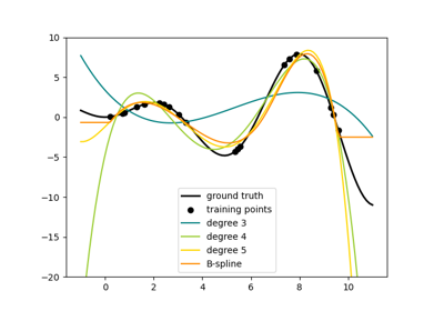
Plotting polynomial regressions with std errors of the scores#
ax = sns.scatterplot(
    data=full_data, x="input_feature", y="target", color="black", alpha=0.75
)
ax.plot(X_plot, y_plot, color="black", label="Ground Truth")
ax.plot(X_plot, y_brr, color="red", label="BayesianRidge with polynomial features")
ax.plot(X_plot, y_ard, color="navy", label="ARD with polynomial features")
ax.fill_between(
    X_plot.ravel(),
    y_ard - y_ard_std,
    y_ard + y_ard_std,
    color="navy",
    alpha=0.3,
)
ax.fill_between(
    X_plot.ravel(),
    y_brr - y_brr_std,
    y_brr + y_brr_std,
    color="red",
    alpha=0.3,
)
ax.legend()
_ = ax.set_title("Polynomial fit of a non-linear feature")
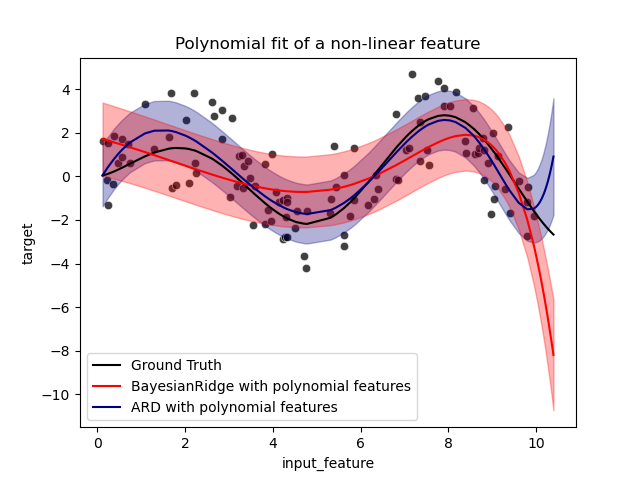
The error bars represent one standard deviation of the predicted gaussian
distribution of the query points. Notice that the ARD regression captures the
ground truth the best when using the default parameters in both models, but
further reducing the lambda_init hyperparameter of the Bayesian Ridge can
reduce its bias (see example
Curve Fitting with Bayesian Ridge Regression).
Finally, due to the intrinsic limitations of a polynomial regression, both
models fail when extrapolating.
Total running time of the script: (0 minutes 0.570 seconds)
Related examples
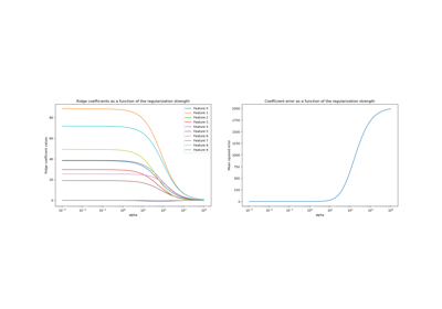
Ridge coefficients as a function of the L2 Regularization
