2.5. Decomposing signals in components (matrix factorization problems)#
2.5.1. Principal component analysis (PCA)#
2.5.1.1. Exact PCA and probabilistic interpretation#
PCA is used to decompose a multivariate dataset in a set of successive
orthogonal components that explain a maximum amount of the variance. In
scikit-learn, PCA is implemented as a transformer object
that learns \(n\) components in its fit method, and can be used on new
data to project it on these components.
PCA centers but does not scale the input data for each feature before
applying the SVD. The optional parameter whiten=True makes it
possible to project the data onto the singular space while scaling each
component to unit variance. This is often useful if the models down-stream make
strong assumptions on the isotropy of the signal: this is for example the case
for Support Vector Machines with the RBF kernel and the K-Means clustering
algorithm.
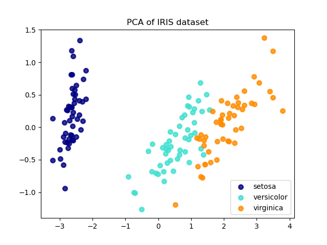
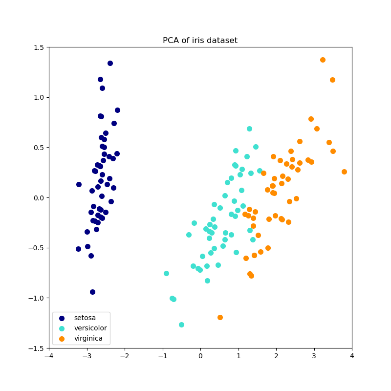
Below is an example of the iris dataset, which is comprised of 4 features, projected on the 2 dimensions that explain most variance:
The PCA object also provides a
probabilistic interpretation of the PCA that can give a likelihood of
data based on the amount of variance it explains. As such it implements a
score method that can be used in cross-validation:
Examples
2.5.1.2. Incremental PCA#
The PCA object is very useful, but has certain limitations for
large datasets. The biggest limitation is that PCA only supports
batch processing, which means all of the data to be processed must fit in main
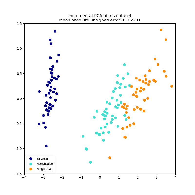
memory. The IncrementalPCA object uses a different form of
processing and allows for partial computations which almost
exactly match the results of PCA while processing the data in a
minibatch fashion. IncrementalPCA makes it possible to implement
out-of-core Principal Component Analysis either by:
Using its
partial_fitmethod on chunks of data fetched sequentially from the local hard drive or a network database.Calling its fit method on a memory mapped file using
numpy.memmap.
IncrementalPCA only stores estimates of component and noise variances,
in order to update explained_variance_ratio_ incrementally. This is why
memory usage depends on the number of samples per batch, rather than the
number of samples to be processed in the dataset.
As in PCA, IncrementalPCA centers but does not scale the
input data for each feature before applying the SVD.
Examples
2.5.1.3. PCA using randomized SVD#
It is often interesting to project data to a lower-dimensional space that preserves most of the variance, by dropping the singular vector of components associated with lower singular values.
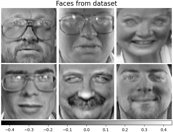
For instance, if we work with 64x64 pixel gray-level pictures for face recognition, the dimensionality of the data is 4096 and it is slow to train an RBF support vector machine on such wide data. Furthermore we know that the intrinsic dimensionality of the data is much lower than 4096 since all pictures of human faces look somewhat alike. The samples lie on a manifold of much lower dimension (say around 200 for instance). The PCA algorithm can be used to linearly transform the data while both reducing the dimensionality and preserving most of the explained variance at the same time.
The class PCA used with the optional parameter
svd_solver='randomized' is very useful in that case: since we are going
to drop most of the singular vectors it is much more efficient to limit the
computation to an approximated estimate of the singular vectors we will keep
to actually perform the transform.
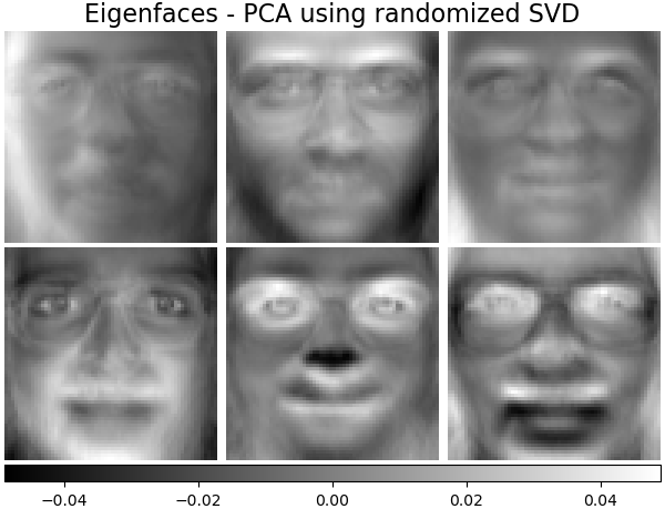
For instance, the following shows 16 sample portraits (centered around 0.0) from the Olivetti dataset. On the right hand side are the first 16 singular vectors reshaped as portraits. Since we only require the top 16 singular vectors of a dataset with size \(n_{samples} = 400\) and \(n_{features} = 64 \times 64 = 4096\), the computation time is less than 1s:
If we note \(n_{\max} = \max(n_{\mathrm{samples}}, n_{\mathrm{features}})\) and
\(n_{\min} = \min(n_{\mathrm{samples}}, n_{\mathrm{features}})\), the time complexity
of the randomized PCA is \(O(n_{\max}^2 \cdot n_{\mathrm{components}})\)
instead of \(O(n_{\max}^2 \cdot n_{\min})\) for the exact method
implemented in PCA.
The memory footprint of randomized PCA is also proportional to
\(2 \cdot n_{\max} \cdot n_{\mathrm{components}}\) instead of \(n_{\max}
\cdot n_{\min}\) for the exact method.
Note: the implementation of inverse_transform in PCA with
svd_solver='randomized' is not the exact inverse transform of
transform even when whiten=False (default).
Examples
References
Algorithm 4.3 in “Finding structure with randomness: Stochastic algorithms for constructing approximate matrix decompositions” Halko, et al., 2009
“An implementation of a randomized algorithm for principal component analysis” A. Szlam et al. 2014
2.5.1.4. Sparse principal components analysis (SparsePCA and MiniBatchSparsePCA)#
SparsePCA is a variant of PCA, with the goal of extracting the
set of sparse components that best reconstruct the data.
Mini-batch sparse PCA (MiniBatchSparsePCA) is a variant of
SparsePCA that is faster but less accurate. The increased speed is
reached by iterating over small chunks of the set of features, for a given
number of iterations.
Principal component analysis (PCA) has the disadvantage that the
components extracted by this method have exclusively dense expressions, i.e.
they have non-zero coefficients when expressed as linear combinations of the
original variables. This can make interpretation difficult. In many cases,
the real underlying components can be more naturally imagined as sparse
vectors; for example in face recognition, components might naturally map to
parts of faces.
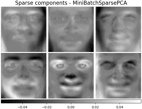
Sparse principal components yield a more parsimonious, interpretable representation, clearly emphasizing which of the original features contribute to the differences between samples.
The following example illustrates 16 components extracted using sparse PCA from the Olivetti faces dataset. It can be seen how the regularization term induces many zeros. Furthermore, the natural structure of the data causes the non-zero coefficients to be vertically adjacent. The model does not enforce this mathematically: each component is a vector \(h \in \mathbf{R}^{4096}\), and there is no notion of vertical adjacency except during the human-friendly visualization as 64x64 pixel images. The fact that the components shown below appear local is the effect of the inherent structure of the data, which makes such local patterns minimize reconstruction error. There exist sparsity-inducing norms that take into account adjacency and different kinds of structure; see [Jen09] for a review of such methods. For more details on how to use Sparse PCA, see the Examples section, below.
Note that there are many different formulations for the Sparse PCA problem. The one implemented here is based on [Mrl09] . The optimization problem solved is a PCA problem (dictionary learning) with an \(\ell_1\) penalty on the components:
\(||.||_{\text{Fro}}\) stands for the Frobenius norm and \(||.||_{1,1}\)
stands for the entry-wise matrix norm which is the sum of the absolute values
of all the entries in the matrix.
The sparsity-inducing \(||.||_{1,1}\) matrix norm also prevents learning
components from noise when few training samples are available. The degree
of penalization (and thus sparsity) can be adjusted through the
hyperparameter alpha. Small values lead to a gently regularized
factorization, while larger values shrink many coefficients to zero.
Note
While in the spirit of an online algorithm, the class
MiniBatchSparsePCA does not implement partial_fit because
the algorithm is online along the features direction, not the samples
direction.
Examples
References
“Online Dictionary Learning for Sparse Coding” J. Mairal, F. Bach, J. Ponce, G. Sapiro, 2009
“Structured Sparse Principal Component Analysis” R. Jenatton, G. Obozinski, F. Bach, 2009
2.5.2. Kernel Principal Component Analysis (kPCA)#
2.5.2.1. Exact Kernel PCA#
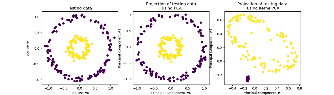
KernelPCA is an extension of PCA which achieves non-linear
dimensionality reduction through the use of kernels (see Pairwise metrics, Affinities and Kernels) [Scholkopf1997]. It
has many applications including denoising, compression and structured
prediction (kernel dependency estimation). KernelPCA supports both
transform and inverse_transform.
Note
KernelPCA.inverse_transform relies on a kernel ridge to learn the
function mapping samples from the PCA basis into the original feature
space [Bakir2003]. Thus, the reconstruction obtained with
KernelPCA.inverse_transform is an approximation. See the example
linked below for more details.
Examples
References
Schölkopf, Bernhard, Alexander Smola, and Klaus-Robert Müller. “Kernel principal component analysis.” International conference on artificial neural networks. Springer, Berlin, Heidelberg, 1997.
Bakır, Gökhan H., Jason Weston, and Bernhard Schölkopf. “Learning to find pre-images.” Advances in neural information processing systems 16 (2003): 449-456.
2.5.2.2. Choice of solver for Kernel PCA#
While in PCA the number of components is bounded by the number of
features, in KernelPCA the number of components is bounded by the
number of samples. Many real-world datasets have large number of samples! In
these cases finding all the components with a full kPCA is a waste of
computation time, as data is mostly described by the first few components
(e.g. n_components<=100). In other words, the centered Gram matrix that
is eigendecomposed in the Kernel PCA fitting process has an effective rank that
is much smaller than its size. This is a situation where approximate
eigensolvers can provide speedup with very low precision loss.
Eigensolvers#
The optional parameter eigen_solver='randomized' can be used to
significantly reduce the computation time when the number of requested
n_components is small compared with the number of samples. It relies on
randomized decomposition methods to find an approximate solution in a shorter
time.
The time complexity of the randomized KernelPCA is
\(O(n_{\mathrm{samples}}^2 \cdot n_{\mathrm{components}})\)
instead of \(O(n_{\mathrm{samples}}^3)\) for the exact method
implemented with eigen_solver='dense'.
The memory footprint of randomized KernelPCA is also proportional to
\(2 \cdot n_{\mathrm{samples}} \cdot n_{\mathrm{components}}\) instead of
\(n_{\mathrm{samples}}^2\) for the exact method.
Note: this technique is the same as in PCA using randomized SVD.
In addition to the above two solvers, eigen_solver='arpack' can be used as
an alternate way to get an approximate decomposition. In practice, this method
only provides reasonable execution times when the number of components to find
is extremely small. It is enabled by default when the desired number of
components is less than 10 (strict) and the number of samples is more than 200
(strict). See KernelPCA for details.
References
dense solver: scipy.linalg.eigh documentation
randomized solver:
Algorithm 4.3 in “Finding structure with randomness: Stochastic algorithms for constructing approximate matrix decompositions” Halko, et al. (2009)
“An implementation of a randomized algorithm for principal component analysis” A. Szlam et al. (2014)
arpack solver: scipy.sparse.linalg.eigsh documentation R. B. Lehoucq, D. C. Sorensen, and C. Yang, (1998)
2.5.3. Truncated singular value decomposition and latent semantic analysis#
TruncatedSVD implements a variant of singular value decomposition
(SVD) that only computes the \(k\) largest singular values,
where \(k\) is a user-specified parameter.
TruncatedSVD is very similar to PCA, but differs
in that the matrix \(X\) does not need to be centered.
When the columnwise (per-feature) means of \(X\)
are subtracted from the feature values,
truncated SVD on the resulting matrix is equivalent to PCA.
About truncated SVD and latent semantic analysis (LSA)#
When truncated SVD is applied to term-document matrices
(as returned by CountVectorizer or
TfidfVectorizer),
this transformation is known as
latent semantic analysis
(LSA), because it transforms such matrices
to a “semantic” space of low dimensionality.
In particular, LSA is known to combat the effects of synonymy and polysemy
(both of which roughly mean there are multiple meanings per word),
which cause term-document matrices to be overly sparse
and exhibit poor similarity under measures such as cosine similarity.
Note
LSA is also known as latent semantic indexing, LSI, though strictly that refers to its use in persistent indexes for information retrieval purposes.
Mathematically, truncated SVD applied to training samples \(X\) produces a low-rank approximation \(X\):
After this operation, \(U_k \Sigma_k\)
is the transformed training set with \(k\) features
(called n_components in the API).
To also transform a test set \(X\), we multiply it with \(V_k\):
Note
Most treatments of LSA in the natural language processing (NLP)
and information retrieval (IR) literature
swap the axes of the matrix \(X\) so that it has shape
(n_features, n_samples).
We present LSA in a different way that matches the scikit-learn API better,
but the singular values found are the same.
While the TruncatedSVD transformer
works with any feature matrix,
using it on tf-idf matrices is recommended over raw frequency counts
in an LSA/document processing setting.
In particular, sublinear scaling and inverse document frequency
should be turned on (sublinear_tf=True, use_idf=True)
to bring the feature values closer to a Gaussian distribution,
compensating for LSA’s erroneous assumptions about textual data.
Examples
References
Christopher D. Manning, Prabhakar Raghavan and Hinrich Schütze (2008), Introduction to Information Retrieval, Cambridge University Press, chapter 18: Matrix decompositions & latent semantic indexing
2.5.4. Dictionary Learning#
2.5.4.1. Sparse coding with a precomputed dictionary#
The SparseCoder object is an estimator that can be used to transform signals
into sparse linear combination of atoms from a fixed, precomputed dictionary
such as a discrete wavelet basis. This object therefore does not
implement a fit method. The transformation amounts
to a sparse coding problem: finding a representation of the data as a linear
combination of as few dictionary atoms as possible. All variations of
dictionary learning implement the following transform methods, controllable via
the transform_method initialization parameter:
Orthogonal matching pursuit (Orthogonal Matching Pursuit (OMP))
Least-angle regression (Least Angle Regression)
Lasso computed by least-angle regression
Lasso using coordinate descent (Lasso)
Thresholding
Thresholding is very fast but it does not yield accurate reconstructions. They have been shown useful in literature for classification tasks. For image reconstruction tasks, orthogonal matching pursuit yields the most accurate, unbiased reconstruction.
The dictionary learning objects offer, via the split_code parameter, the
possibility to separate the positive and negative values in the results of
sparse coding. This is useful when dictionary learning is used for extracting
features that will be used for supervised learning, because it allows the
learning algorithm to assign different weights to negative loadings of a
particular atom, from to the corresponding positive loading.
The split code for a single sample has length 2 * n_components
and is constructed using the following rule: First, the regular code of length
n_components is computed. Then, the first n_components entries of the
split_code are
filled with the positive part of the regular code vector. The second half of
the split code is filled with the negative part of the code vector, only with
a positive sign. Therefore, the split_code is non-negative.
Examples
2.5.4.2. Generic dictionary learning#
Dictionary learning (DictionaryLearning) is a matrix factorization
problem that amounts to finding a (usually overcomplete) dictionary that will
perform well at sparsely encoding the fitted data.
Representing data as sparse combinations of atoms from an overcomplete dictionary is suggested to be the way the mammalian primary visual cortex works. Consequently, dictionary learning applied on image patches has been shown to give good results in image processing tasks such as image completion, inpainting and denoising, as well as for supervised recognition tasks.
Dictionary learning is an optimization problem solved by alternatively updating the sparse code, as a solution to multiple Lasso problems, considering the dictionary fixed, and then updating the dictionary to best fit the sparse code.
\(||.||_{\text{Fro}}\) stands for the Frobenius norm and \(||.||_{1,1}\) stands for the entry-wise matrix norm which is the sum of the absolute values of all the entries in the matrix. After using such a procedure to fit the dictionary, the transform is simply a sparse coding step that shares the same implementation with all dictionary learning objects (see Sparse coding with a precomputed dictionary).
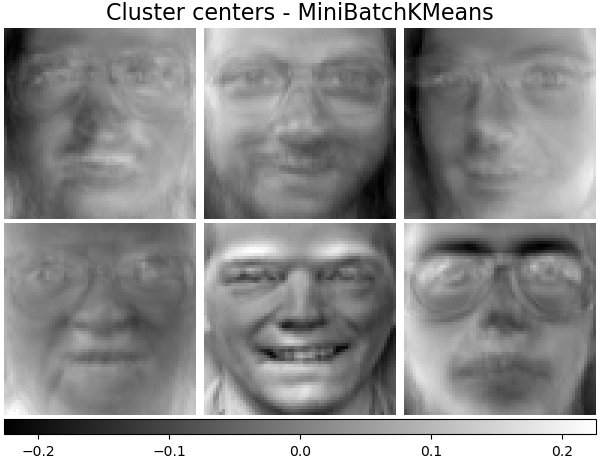
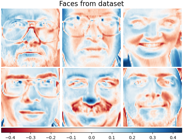
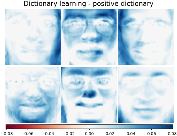
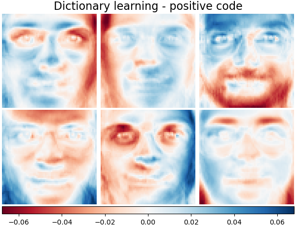
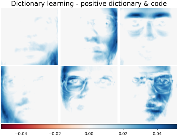
It is also possible to constrain the dictionary and/or code to be positive to match constraints that may be present in the data. Below are the faces with different positivity constraints applied. Red indicates negative values, blue indicates positive values, and white represents zeros.
References
“Online dictionary learning for sparse coding” J. Mairal, F. Bach, J. Ponce, G. Sapiro, 2009
2.5.4.3. Mini-batch dictionary learning#
MiniBatchDictionaryLearning implements a faster, but less accurate
version of the dictionary learning algorithm that is better suited for large
datasets.
By default, MiniBatchDictionaryLearning divides the data into
mini-batches and optimizes in an online manner by cycling over the mini-batches
for the specified number of iterations. However, at the moment it does not
implement a stopping condition.
The estimator also implements partial_fit, which updates the dictionary by
iterating only once over a mini-batch. This can be used for online learning
when the data is not readily available from the start, or for when the data
does not fit into memory.
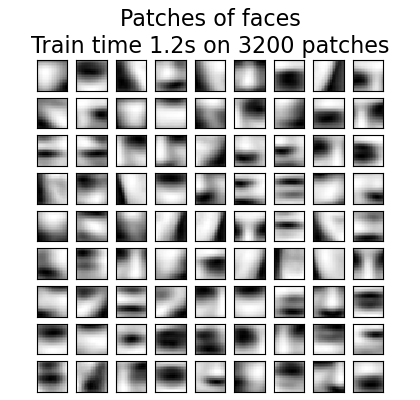
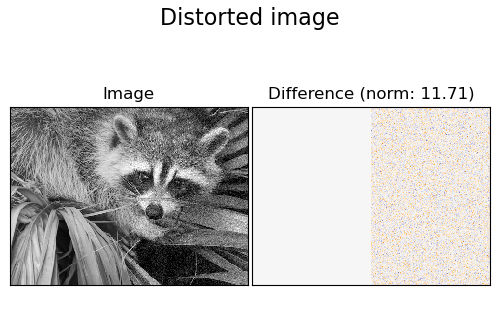
The following image shows how a dictionary, learned from 4x4 pixel image patches extracted from part of the image of a raccoon face, looks like.
Examples
2.5.5. Factor Analysis#
In unsupervised learning we only have a dataset \(X = \{x_1, x_2, \dots, x_n
\}\). How can this dataset be described mathematically? A very simple
continuous latent variable model for \(X\) is
The vector \(h_i\) is called “latent” because it is unobserved. \(\epsilon\) is considered a noise term distributed according to a Gaussian with mean 0 and covariance \(\Psi\) (i.e. \(\epsilon \sim \mathcal{N}(0, \Psi)\)), \(\mu\) is some arbitrary offset vector. Such a model is called “generative” as it describes how \(x_i\) is generated from \(h_i\). If we use all the \(x_i\)’s as columns to form a matrix \(\mathbf{X}\) and all the \(h_i\)’s as columns of a matrix \(\mathbf{H}\) then we can write (with suitably defined \(\mathbf{M}\) and \(\mathbf{E}\)):
In other words, we decomposed matrix \(\mathbf{X}\).
If \(h_i\) is given, the above equation automatically implies the following probabilistic interpretation:
For a complete probabilistic model we also need a prior distribution for the latent variable \(h\). The most straightforward assumption (based on the nice properties of the Gaussian distribution) is \(h \sim \mathcal{N}(0, \mathbf{I})\). This yields a Gaussian as the marginal distribution of \(x\):
Now, without any further assumptions the idea of having a latent variable \(h\) would be superfluous – \(x\) can be completely modelled with a mean and a covariance. We need to impose some more specific structure on one of these two parameters. A simple additional assumption regards the structure of the error covariance \(\Psi\):
\(\Psi = \sigma^2 \mathbf{I}\): This assumption leads to the probabilistic model of
PCA.\(\Psi = \mathrm{diag}(\psi_1, \psi_2, \dots, \psi_n)\): This model is called
FactorAnalysis, a classical statistical model. The matrix W is sometimes called the “factor loading matrix”.
Both models essentially estimate a Gaussian with a low-rank covariance matrix.
Because both models are probabilistic they can be integrated in more complex
models, e.g. Mixture of Factor Analysers. One gets very different models (e.g.
FastICA) if non-Gaussian priors on the latent variables are assumed.
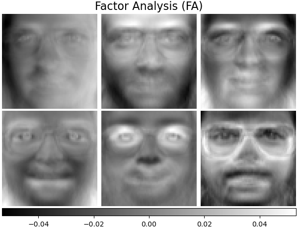
Factor analysis can produce similar components (the columns of its loading
matrix) to PCA. However, one can not make any general statements
about these components (e.g. whether they are orthogonal):
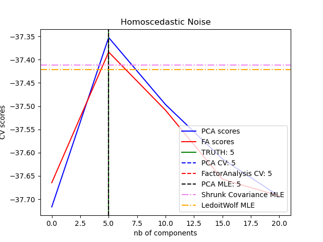
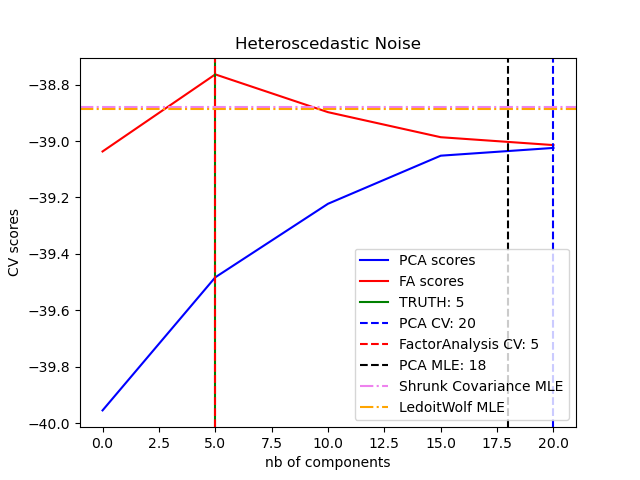
The main advantage for Factor Analysis over PCA is that
it can model the variance in every direction of the input space independently
(heteroscedastic noise):
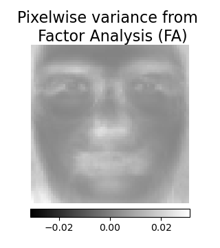
This allows better model selection than probabilistic PCA in the presence of heteroscedastic noise:
Factor Analysis is often followed by a rotation of the factors (with the
parameter rotation), usually to improve interpretability. For example,
Varimax rotation maximizes the sum of the variances of the squared loadings,
i.e., it tends to produce sparser factors, which are influenced by only a few
features each (the “simple structure”). See e.g., the first example below.
Examples
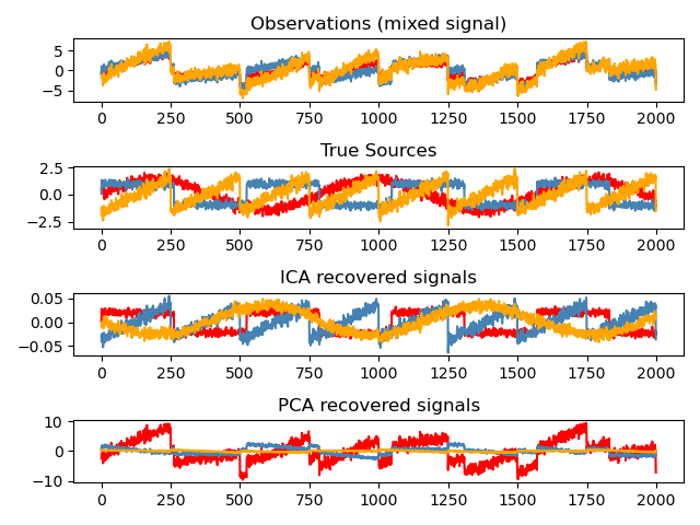
2.5.6. Independent component analysis (ICA)#
Independent component analysis separates a multivariate signal into
additive subcomponents that are maximally independent. It is
implemented in scikit-learn using the Fast ICA
algorithm. Typically, ICA is not used for reducing dimensionality but
for separating superimposed signals. Since the ICA model does not include
a noise term, for the model to be correct, whitening must be applied.
This can be done internally using the whiten argument or manually using one
of the PCA variants.
It is classically used to separate mixed signals (a problem known as blind source separation), as in the example below:
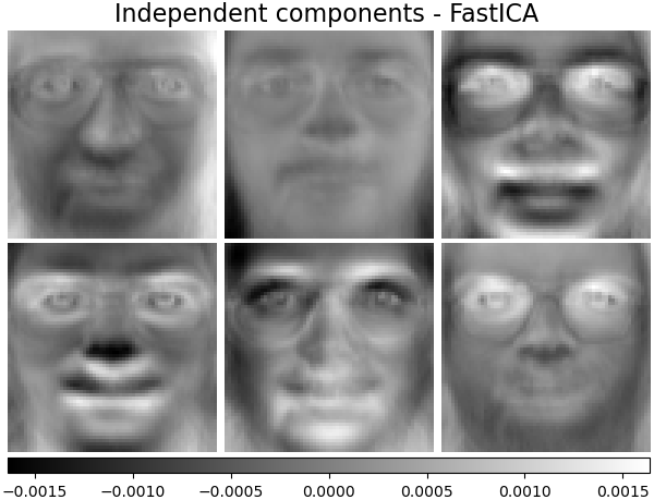
ICA can also be used as yet another non linear decomposition that finds components with some sparsity:
Examples
2.5.7. Non-negative matrix factorization (NMF or NNMF)#
2.5.7.1. NMF with the Frobenius norm#
NMF [1] is an alternative approach to decomposition that assumes that the
data and the components are non-negative. NMF can be plugged in
instead of PCA or its variants, in the cases where the data matrix
does not contain negative values. It finds a decomposition of samples
\(X\) into two matrices \(W\) and \(H\) of non-negative elements,
by optimizing the distance \(d\) between \(X\) and the matrix product
\(WH\). The most widely used distance function is the squared Frobenius
norm, which is an obvious extension of the Euclidean norm to matrices:
Unlike PCA, the representation of a vector is obtained in an additive
fashion, by superimposing the components, without subtracting. Such additive
models are efficient for representing images and text.
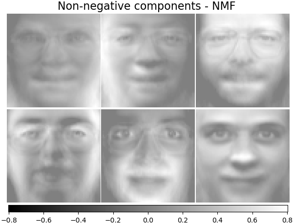
It has been observed in [Hoyer, 2004] [2] that, when carefully constrained,
NMF can produce a parts-based representation of the dataset,
resulting in interpretable models. The following example displays 16
sparse components found by NMF from the images in the Olivetti
faces dataset, in comparison with the PCA eigenfaces.
The init attribute determines the initialization method applied, which
has a great impact on the performance of the method. NMF implements the
method Nonnegative Double Singular Value Decomposition. NNDSVD [4] is based on
two SVD processes, one approximating the data matrix, the other approximating
positive sections of the resulting partial SVD factors utilizing an algebraic
property of unit rank matrices. The basic NNDSVD algorithm is better fit for
sparse factorization. Its variants NNDSVDa (in which all zeros are set equal to
the mean of all elements of the data), and NNDSVDar (in which the zeros are set
to random perturbations less than the mean of the data divided by 100) are
recommended in the dense case.
Note that the Multiplicative Update (‘mu’) solver cannot update zeros present in the initialization, so it leads to poorer results when used jointly with the basic NNDSVD algorithm which introduces a lot of zeros; in this case, NNDSVDa or NNDSVDar should be preferred.
NMF can also be initialized with correctly scaled random non-negative
matrices by setting init="random". An integer seed or a
RandomState can also be passed to random_state to control
reproducibility.
In NMF, L1 and L2 priors can be added to the loss function in order to
regularize the model. The L2 prior uses the Frobenius norm, while the L1 prior
uses an elementwise L1 norm. As in ElasticNet,
we control the combination of L1 and L2 with the l1_ratio (\(\rho\))
parameter, and the intensity of the regularization with the alpha_W and
alpha_H (\(\alpha_W\) and \(\alpha_H\)) parameters. The priors are
scaled by the number of samples (\(n\_samples\)) for H and the number of
features (\(n\_features\)) for W to keep their impact balanced with
respect to one another and to the data fit term as independent as possible of
the size of the training set. Then the priors terms are:
and the regularized objective function is:
2.5.7.2. NMF with a beta-divergence#
As described previously, the most widely used distance function is the squared Frobenius norm, which is an obvious extension of the Euclidean norm to matrices:
Other distance functions can be used in NMF as, for example, the (generalized) Kullback-Leibler (KL) divergence, also referred as I-divergence:
Or, the Itakura-Saito (IS) divergence:
These three distances are special cases of the beta-divergence family, with \(\beta = 2, 1, 0\) respectively [6]. The beta-divergence is defined by :
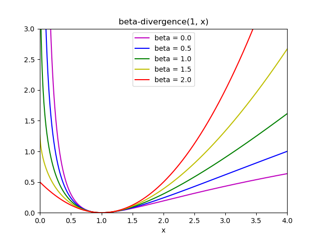
Note that this definition is not valid if \(\beta \in (0; 1)\), yet it can be continuously extended to the definitions of \(d_{KL}\) and \(d_{IS}\) respectively.
NMF implemented solvers#
NMF implements two solvers, using Coordinate Descent (‘cd’) [5], and
Multiplicative Update (‘mu’) [6]. The ‘mu’ solver can optimize every
beta-divergence, including of course the Frobenius norm (\(\beta=2\)), the
(generalized) Kullback-Leibler divergence (\(\beta=1\)) and the
Itakura-Saito divergence (\(\beta=0\)). Note that for
\(\beta \in (1; 2)\), the ‘mu’ solver is significantly faster than for other
values of \(\beta\). Note also that with a negative (or 0, i.e.
‘itakura-saito’) \(\beta\), the input matrix cannot contain zero values.
The ‘cd’ solver can only optimize the Frobenius norm. Due to the underlying non-convexity of NMF, the different solvers may converge to different minima, even when optimizing the same distance function.
NMF is best used with the fit_transform method, which returns the matrix W.
The matrix H is stored into the fitted model in the components_ attribute;
the method transform will decompose a new matrix X_new based on these
stored components:
>>> import numpy as np
>>> X = np.array([[1, 1], [2, 1], [3, 1.2], [4, 1], [5, 0.8], [6, 1]])
>>> from sklearn.decomposition import NMF
>>> model = NMF(n_components=2, init='random', random_state=0)
>>> W = model.fit_transform(X)
>>> H = model.components_
>>> X_new = np.array([[1, 0], [1, 6.1], [1, 0], [1, 4], [3.2, 1], [0, 4]])
>>> W_new = model.transform(X_new)
Examples
2.5.7.3. Mini-batch Non Negative Matrix Factorization#
MiniBatchNMF [7] implements a faster, but less accurate version of the
non negative matrix factorization (i.e. NMF),
better suited for large datasets.
By default, MiniBatchNMF divides the data into mini-batches and
optimizes the NMF model in an online manner by cycling over the mini-batches
for the specified number of iterations. The batch_size parameter controls
the size of the batches.
In order to speed up the mini-batch algorithm it is also possible to scale
past batches, giving them less importance than newer batches. This is done
by introducing a so-called forgetting factor controlled by the forget_factor
parameter.
The estimator also implements partial_fit, which updates H by iterating
only once over a mini-batch. This can be used for online learning when the data
is not readily available from the start, or when the data does not fit into memory.
References
2.5.8. Latent Dirichlet Allocation (LDA)#
Latent Dirichlet Allocation is a generative probabilistic model for collections of discrete datasets such as text corpora. It is also a topic model that is used for discovering abstract topics from a collection of documents.
The graphical model of LDA is a three-level generative model:

Note on notations presented in the graphical model above, which can be found in Hoffman et al. (2013):
The corpus is a collection of \(D\) documents.
A document \(d \in D\) is a sequence of \(N_d\) words.
There are \(K\) topics in the corpus.
The boxes represent repeated sampling.
In the graphical model, each node is a random variable and has a role in the generative process. A shaded node indicates an observed variable and an unshaded node indicates a hidden (latent) variable. In this case, words in the corpus are the only data that we observe. The latent variables determine the random mixture of topics in the corpus and the distribution of words in the documents. The goal of LDA is to use the observed words to infer the hidden topic structure.
Details on modeling text corpora#
When modeling text corpora, the model assumes the following generative process
for a corpus with \(D\) documents and \(K\) topics, with \(K\)
corresponding to n_components in the API:
For each topic \(k \in K\), draw \(\beta_k \sim \mathrm{Dirichlet}(\eta)\). This provides a distribution over the words, i.e. the probability of a word appearing in topic \(k\). \(\eta\) corresponds to
topic_word_prior.For each document \(d \in D\), draw the topic proportions \(\theta_d \sim \mathrm{Dirichlet}(\alpha)\). \(\alpha\) corresponds to
doc_topic_prior.For each word \(n=1,\cdots,N_d\) in document \(d\):
Draw the topic assignment \(z_{dn} \sim \mathrm{Multinomial} (\theta_d)\)
Draw the observed word \(w_{dn} \sim \mathrm{Multinomial} (\beta_{z_{dn}})\)
For parameter estimation, the posterior distribution is:
Since the posterior is intractable, variational Bayesian method uses a simpler distribution \(q(z,\theta,\beta | \lambda, \phi, \gamma)\) to approximate it, and those variational parameters \(\lambda\), \(\phi\), \(\gamma\) are optimized to maximize the Evidence Lower Bound (ELBO):
Maximizing ELBO is equivalent to minimizing the Kullback-Leibler(KL) divergence between \(q(z,\theta,\beta)\) and the true posterior \(p(z, \theta, \beta |w, \alpha, \eta)\).
LatentDirichletAllocation implements the online variational Bayes
algorithm and supports both online and batch update methods.
While the batch method updates variational variables after each full pass through
the data, the online method updates variational variables from mini-batch data
points.
Note
Although the online method is guaranteed to converge to a local optimum point, the quality of the optimum point and the speed of convergence may depend on mini-batch size and attributes related to learning rate setting.
When LatentDirichletAllocation is applied on a “document-term” matrix, the matrix
will be decomposed into a “topic-term” matrix and a “document-topic” matrix. While
“topic-term” matrix is stored as components_ in the model, “document-topic” matrix
can be calculated from transform method.
LatentDirichletAllocation also implements partial_fit method. This is used
when data can be fetched sequentially.
Examples
References
“Latent Dirichlet Allocation” D. Blei, A. Ng, M. Jordan, 2003
“Online Learning for Latent Dirichlet Allocation” M. Hoffman, D. Blei, F. Bach, 2010
“Stochastic Variational Inference” M. Hoffman, D. Blei, C. Wang, J. Paisley, 2013
“The varimax criterion for analytic rotation in factor analysis” H. F. Kaiser, 1958
See also Dimensionality reduction for dimensionality reduction with Neighborhood Components Analysis.
