1.14. Semi-supervised learning#
Semi-supervised learning is a situation
in which in your training data some of the samples are not labeled. The
semi-supervised estimators in sklearn.semi_supervised are able to
make use of this additional unlabeled data to better capture the shape of
the underlying data distribution and generalize better to new samples.
These algorithms can perform well when we have a very small amount of
labeled points and a large amount of unlabeled points.
Note
Semi-supervised algorithms need to make assumptions about the distribution of the dataset in order to achieve performance gains. See here for more details.
Examples
1.14.1. Self Training#
This self-training implementation is based on Yarowsky’s [1] algorithm. Using this algorithm, a given supervised classifier can function as a semi-supervised classifier, allowing it to learn from unlabeled data.
SelfTrainingClassifier can be called with any classifier that
implements predict_proba, passed as the parameter estimator. In
each iteration, the estimator predicts labels for the unlabeled
samples and adds a subset of these labels to the labeled dataset.
The choice of this subset is determined by the selection criterion. This
selection can be done using a threshold on the prediction probabilities, or
by choosing the k_best samples according to the prediction probabilities.
The labels used for the final fit as well as the iteration in which each sample
was labeled are available as attributes. The optional max_iter parameter
specifies how many times the loop is executed at most.
The max_iter parameter may be set to None, causing the algorithm to iterate
until all samples have labels or no new samples are selected in that iteration.
Note
When using the self-training classifier, the calibration of the classifier is important.
Examples
References
1.14.2. Label Propagation#
Label propagation denotes a few variations of semi-supervised graph inference algorithms.
- A few features available in this model:
Used for classification tasks
Kernel methods to project data into alternate dimensional spaces
scikit-learn provides two label propagation models:
LabelPropagation and LabelSpreading. Both work by
constructing a similarity graph over all items in the input dataset.
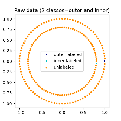
An illustration of label-propagation: the structure of unlabeled observations is consistent with the class structure, and thus the class label can be propagated to the unlabeled observations of the training set.#
LabelPropagation and LabelSpreading
differ in modifications to the similarity matrix that graph and the
clamping effect on the label distributions.
Clamping allows the algorithm to change the weight of the true ground labeled
data to some degree. The LabelPropagation algorithm performs hard
clamping of input labels, which means \(\alpha=0\). This clamping factor
can be relaxed, to say \(\alpha=0.2\), which means that we will always
retain 80 percent of our original label distribution, but the algorithm gets to
change its confidence of the distribution within 20 percent.
LabelPropagation uses the raw similarity matrix constructed from
the data with no modifications. In contrast, LabelSpreading
minimizes a loss function that has regularization properties, as such it
is often more robust to noise. The algorithm iterates on a modified
version of the original graph and normalizes the edge weights by
computing the normalized graph Laplacian matrix. This procedure is also
used in Spectral clustering.
Label propagation models have two built-in kernel methods. Choice of kernel affects both scalability and performance of the algorithms. The following are available:
rbf (\(\exp(-\gamma |x-y|^2), \gamma > 0\)). \(\gamma\) is specified by keyword gamma.
knn (\(1[x' \in kNN(x)]\)). \(k\) is specified by keyword n_neighbors.
The RBF kernel will produce a fully connected graph which is represented in memory by a dense matrix. This matrix may be very large and combined with the cost of performing a full matrix multiplication calculation for each iteration of the algorithm can lead to prohibitively long running times. On the other hand, the KNN kernel will produce a much more memory-friendly sparse matrix which can drastically reduce running times.
Examples
References
[2] Yoshua Bengio, Olivier Delalleau, Nicolas Le Roux. In Semi-Supervised Learning (2006), pp. 193-216
[3] Olivier Delalleau, Yoshua Bengio, Nicolas Le Roux. Efficient Non-Parametric Function Induction in Semi-Supervised Learning. AISTAT 2005 https://www.gatsby.ucl.ac.uk/aistats/fullpapers/204.pdf
