spectral_clustering#
- sklearn.cluster.spectral_clustering(affinity, *, n_clusters=8, n_components=None, eigen_solver=None, random_state=None, n_init=10, eigen_tol='auto', assign_labels='kmeans', verbose=False)[source]#
Apply clustering to a projection of the normalized Laplacian.
In practice Spectral Clustering is very useful when the structure of the individual clusters is highly non-convex or more generally when a measure of the center and spread of the cluster is not a suitable description of the complete cluster. For instance, when clusters are nested circles on the 2D plane.
If affinity is the adjacency matrix of a graph, this method can be used to find normalized graph cuts [1], [2].
Read more in the User Guide.
- Parameters:
- affinity{array-like, sparse matrix} of shape (n_samples, n_samples)
The affinity matrix describing the relationship of the samples to embed. Must be symmetric.
- Possible examples:
adjacency matrix of a graph,
heat kernel of the pairwise distance matrix of the samples,
symmetric k-nearest neighbours connectivity matrix of the samples.
- n_clustersint, default=None
Number of clusters to extract.
- n_componentsint, default=n_clusters
Number of eigenvectors to use for the spectral embedding.
- eigen_solver{None, ‘arpack’, ‘lobpcg’, or ‘amg’}
The eigenvalue decomposition method. If None then
'arpack'is used. See [4] for more details regarding'lobpcg'. Eigensolver'amg'runs'lobpcg'with optional Algebraic MultiGrid preconditioning and requires pyamg to be installed. It can be faster on very large sparse problems [6] and [7].- random_stateint, RandomState instance, default=None
A pseudo random number generator used for the initialization of the lobpcg eigenvectors decomposition when
eigen_solver ==
'amg'
, and for the K-Means initialization. Use an int to make the results deterministic across calls (See Glossary).Note
When using
eigen_solver == 'amg', it is necessary to also fix the global numpy seed withnp.random.seed(int)to get deterministic results. See pyamg/pyamg#139 for further information.- n_initint, default=10
Number of time the k-means algorithm will be run with different centroid seeds. The final results will be the best output of n_init consecutive runs in terms of inertia. Only used if
assign_labels='kmeans'.- eigen_tolfloat, default=”auto”
Stopping criterion for eigendecomposition of the Laplacian matrix. If
eigen_tol="auto"then the passed tolerance will depend on theeigen_solver:If
eigen_solver="arpack", theneigen_tol=0.0;If
eigen_solver="lobpcg"oreigen_solver="amg", theneigen_tol=Nonewhich configures the underlyinglobpcgsolver to automatically resolve the value according to their heuristics. See,scipy.sparse.linalg.lobpcgfor details.
Note that when using
eigen_solver="lobpcg"oreigen_solver="amg"values oftol<1e-5may lead to convergence issues and should be avoided.Added in version 1.2: Added ‘auto’ option.
- assign_labels{‘kmeans’, ‘discretize’, ‘cluster_qr’}, default=’kmeans’
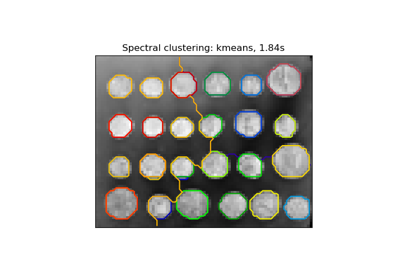
The strategy to use to assign labels in the embedding space. There are three ways to assign labels after the Laplacian embedding. k-means can be applied and is a popular choice. But it can also be sensitive to initialization. Discretization is another approach which is less sensitive to random initialization [3]. The cluster_qr method [5] directly extracts clusters from eigenvectors in spectral clustering. In contrast to k-means and discretization, cluster_qr has no tuning parameters and is not an iterative method, yet may outperform k-means and discretization in terms of both quality and speed. For a detailed comparison of clustering strategies, refer to the following example: Segmenting the picture of greek coins in regions.
Changed in version 1.1: Added new labeling method ‘cluster_qr’.
- verbosebool, default=False
Verbosity mode.
Added in version 0.24.
- Returns:
- labelsarray of integers, shape: n_samples
The labels of the clusters.
Notes
The graph should contain only one connected component, elsewhere the results make little sense.
This algorithm solves the normalized cut for
k=2: it is a normalized spectral clustering.References
Examples
>>> import numpy as np
>>> from sklearn.metrics.pairwise import pairwise_kernels
>>> from sklearn.cluster import spectral_clustering
>>> X = np.array([[1, 1], [2, 1], [1, 0],
...               [4, 7], [3, 5], [3, 6]])
>>> affinity = pairwise_kernels(X, metric='rbf')
>>> spectral_clustering(
...     affinity=affinity, n_clusters=2, assign_labels="discretize", random_state=0
... )
array([1, 1, 1, 0, 0, 0])


