Note

Go to the end to download the full example code. or to run this example in your browser via JupyterLite or Binder

Ordinary Least Squares Example#

This example shows how to use the ordinary least squares (OLS) model called LinearRegression in scikit-learn.

For this purpose, we use a single feature from the diabetes dataset and try to predict the diabetes progression using this linear model. We therefore load the diabetes dataset and split it into training and test sets.

Then, we fit the model on the training set and evaluate its performance on the test set and finally visualize the results on the test set.

# Authors: The scikit-learn developers
# SPDX-License-Identifier: BSD-3-Clause

Data Loading and Preparation#

Load the diabetes dataset. For simplicity, we only keep a single feature in the data. Then, we split the data and target into training and test sets.

from sklearn.datasets import load_diabetes
from sklearn.model_selection import train_test_split

X, y = load_diabetes(return_X_y=True)
X = X[:, [2]]  # Use only one feature
X_train, X_test, y_train, y_test = train_test_split(X, y, test_size=20, shuffle=False)

Linear regression model#

We create a linear regression model and fit it on the training data. Note that by default, an intercept is added to the model. We can control this behavior by setting the fit_intercept parameter.

from sklearn.linear_model import LinearRegression

regressor = LinearRegression().fit(X_train, y_train)

Model evaluation#

We evaluate the model’s performance on the test set using the mean squared error and the coefficient of determination.

from sklearn.metrics import mean_squared_error, r2_score

y_pred = regressor.predict(X_test)

print(f"Mean squared error: {mean_squared_error(y_test, y_pred):.2f}")
print(f"Coefficient of determination: {r2_score(y_test, y_pred):.2f}")

Mean squared error: 2548.07
Coefficient of determination: 0.47

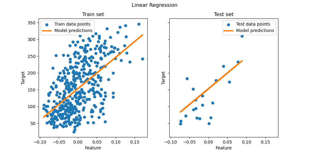
Plotting the results#

Finally, we visualize the results on the train and test data.

import matplotlib.pyplot as plt

fig, ax = plt.subplots(ncols=2, figsize=(10, 5), sharex=True, sharey=True)

ax[0].scatter(X_train, y_train, label="Train data points")
ax[0].plot(
    X_train,
    regressor.predict(X_train),
    linewidth=3,
    color="tab:orange",
    label="Model predictions",
)
ax[0].set(xlabel="Feature", ylabel="Target", title="Train set")
ax[0].legend()

ax[1].scatter(X_test, y_test, label="Test data points")
ax[1].plot(X_test, y_pred, linewidth=3, color="tab:orange", label="Model predictions")
ax[1].set(xlabel="Feature", ylabel="Target", title="Test set")
ax[1].legend()

fig.suptitle("Linear Regression")

plt.show()

Conclusion#

The trained model corresponds to the estimator that minimizes the mean squared error between the predicted and the true target values on the training data. We therefore obtain an estimator of the conditional mean of the target given the data.

Note that in higher dimensions, minimizing only the squared error might lead to overfitting. Therefore, regularization techniques are commonly used to prevent this issue, such as those implemented in Ridge or Lasso.

Total running time of the script: (0 minutes 0.146 seconds)