Note

Go to the end to download the full example code. or to run this example in your browser via JupyterLite or Binder

SVM: Weighted samples#

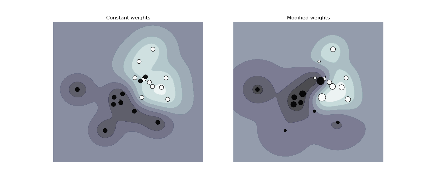
Plot decision function of a weighted dataset, where the size of points is proportional to its weight.

The sample weighting rescales the C parameter, which means that the classifier puts more emphasis on getting these points right. The effect might often be subtle. To emphasize the effect here, we particularly weight outliers, making the deformation of the decision boundary very visible.

# Authors: The scikit-learn developers
# SPDX-License-Identifier: BSD-3-Clause

import matplotlib.pyplot as plt
import numpy as np

from sklearn import svm


def plot_decision_function(classifier, sample_weight, axis, title):
    # plot the decision function
    xx, yy = np.meshgrid(np.linspace(-4, 5, 500), np.linspace(-4, 5, 500))

    Z = classifier.decision_function(np.c_[xx.ravel(), yy.ravel()])
    Z = Z.reshape(xx.shape)

    # plot the line, the points, and the nearest vectors to the plane
    axis.contourf(xx, yy, Z, alpha=0.75, cmap=plt.cm.bone)
    axis.scatter(
        X[:, 0],
        X[:, 1],
        c=y,
        s=100 * sample_weight,
        alpha=0.9,
        cmap=plt.cm.bone,
        edgecolors="black",
    )

    axis.axis("off")
    axis.set_title(title)


# we create 20 points
np.random.seed(0)
X = np.r_[np.random.randn(10, 2) + [1, 1], np.random.randn(10, 2)]
y = [1] * 10 + [-1] * 10
sample_weight_last_ten = abs(np.random.randn(len(X)))
sample_weight_constant = np.ones(len(X))
# and bigger weights to some outliers
sample_weight_last_ten[15:] *= 5
sample_weight_last_ten[9] *= 15

# Fit the models.

# This model does not take into account sample weights.
clf_no_weights = svm.SVC(gamma=1)
clf_no_weights.fit(X, y)

# This other model takes into account some dedicated sample weights.
clf_weights = svm.SVC(gamma=1)
clf_weights.fit(X, y, sample_weight=sample_weight_last_ten)

fig, axes = plt.subplots(1, 2, figsize=(14, 6))
plot_decision_function(
    clf_no_weights, sample_weight_constant, axes[0], "Constant weights"
)
plot_decision_function(clf_weights, sample_weight_last_ten, axes[1], "Modified weights")

plt.show()