Note

Go to the end to download the full example code. or to run this example in your browser via JupyterLite or Binder

Plot classification probability#

Plot the classification probability for different classifiers. We use a 3 class dataset, and we classify it with a Support Vector classifier, L1 and L2 penalized logistic regression (multinomial multiclass), a One-Vs-Rest version with logistic regression, and Gaussian process classification.

Linear SVC is not a probabilistic classifier by default but it has a built-in calibration option enabled in this example (probability=True).

The logistic regression with One-Vs-Rest is not a multiclass classifier out of the box. As a result it has more trouble in separating class 2 and 3 than the other estimators.

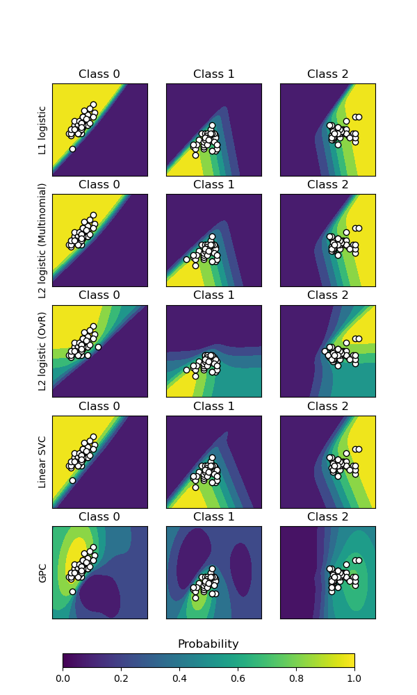
Class 0, Class 1, Class 2, Class 0, Class 1, Class 2, Class 0, Class 1, Class 2, Class 0, Class 1, Class 2, Class 0, Class 1, Class 2, Probability

Accuracy (train) for L1 logistic: 83.3%
Accuracy (train) for L2 logistic (Multinomial): 82.7%
Accuracy (train) for L2 logistic (OvR): 79.3%
Accuracy (train) for Linear SVC: 82.0%
Accuracy (train) for GPC: 82.7%

# Authors: The scikit-learn developers
# SPDX-License-Identifier: BSD-3-Clause

import matplotlib.pyplot as plt
import numpy as np
from matplotlib import cm

from sklearn import datasets
from sklearn.gaussian_process import GaussianProcessClassifier
from sklearn.gaussian_process.kernels import RBF
from sklearn.inspection import DecisionBoundaryDisplay
from sklearn.linear_model import LogisticRegression
from sklearn.metrics import accuracy_score
from sklearn.multiclass import OneVsRestClassifier
from sklearn.svm import SVC

iris = datasets.load_iris()
X = iris.data[:, 0:2]  # we only take the first two features for visualization
y = iris.target

n_features = X.shape[1]

C = 10
kernel = 1.0 * RBF([1.0, 1.0])  # for GPC

# Create different classifiers.
classifiers = {
    "L1 logistic": LogisticRegression(C=C, penalty="l1", solver="saga", max_iter=10000),
    "L2 logistic (Multinomial)": LogisticRegression(
        C=C, penalty="l2", solver="saga", max_iter=10000
    ),
    "L2 logistic (OvR)": OneVsRestClassifier(
        LogisticRegression(C=C, penalty="l2", solver="saga", max_iter=10000)
    ),
    "Linear SVC": SVC(kernel="linear", C=C, probability=True, random_state=0),
    "GPC": GaussianProcessClassifier(kernel),
}

n_classifiers = len(classifiers)

fig, axes = plt.subplots(
    nrows=n_classifiers,
    ncols=len(iris.target_names),
    figsize=(3 * 2, n_classifiers * 2),
)
for classifier_idx, (name, classifier) in enumerate(classifiers.items()):
    y_pred = classifier.fit(X, y).predict(X)
    accuracy = accuracy_score(y, y_pred)
    print(f"Accuracy (train) for {name}: {accuracy:0.1%}")
    for label in np.unique(y):
        # plot the probability estimate provided by the classifier
        disp = DecisionBoundaryDisplay.from_estimator(
            classifier,
            X,
            response_method="predict_proba",
            class_of_interest=label,
            ax=axes[classifier_idx, label],
            vmin=0,
            vmax=1,
        )
        axes[classifier_idx, label].set_title(f"Class {label}")
        # plot data predicted to belong to given class
        mask_y_pred = y_pred == label
        axes[classifier_idx, label].scatter(
            X[mask_y_pred, 0], X[mask_y_pred, 1], marker="o", c="w", edgecolor="k"
        )
        axes[classifier_idx, label].set(xticks=(), yticks=())
    axes[classifier_idx, 0].set_ylabel(name)

ax = plt.axes([0.15, 0.04, 0.7, 0.02])
plt.title("Probability")
_ = plt.colorbar(
    cm.ScalarMappable(norm=None, cmap="viridis"), cax=ax, orientation="horizontal"
)

plt.show()